SELECT
Returns data from a table.
Returns data from a single table. A SELECT statement without a
WHERE clause is not recommended because all rows from all partitions are
returned.
WHERE clause. Queries across multiple partitions can impact
performance.Synopsis
SELECT selectors
  FROM [keyspace_name.]table_name
  [ WHERE [ primary_key_conditions ] [ AND ] [ index_conditions ]
  [ GROUP BY column_name [ , ... ] ]
  [ ORDER BY PK_column_name [ , ... ] ( ASC | DESC ) ]
  [ ( LIMIT N | PER PARTITION LIMIT N ) ]
  [ ALLOW FILTERING ] ;
| Syntax conventions | Description |
|---|---|
| UPPERCASE | Literal keyword. |
| Lowercase | Not literal. |
Italics |
Variable value. Replace with a user-defined value. |
[] |
Optional. Square brackets ( [] ) surround
optional command arguments. Do not type the square brackets. |
( ) |
Group. Parentheses ( ( ) ) identify a group to
choose from. Do not type the parentheses. |
| |
Or. A vertical bar ( | ) separates alternative
elements. Type any one of the elements. Do not type the vertical
bar. |
... |
Repeatable. An ellipsis ( ... ) indicates that
you can repeat the syntax element as often as required. |
'Literal string' |
Single quotation ( ' ) marks must surround
literal strings in CQL statements. Use single quotation marks to
preserve upper case. |
{ key : value
} |
Map collection. Braces ( { } ) enclose map
collections or key value pairs. A colon separates the key and the
value. |
<datatype1,datatype2> |
Set, list, map, or tuple. Angle brackets ( <
> ) enclose data types in a set, list, map, or tuple.
Separate the data types with a comma. |
cql_statement; |
End CQL statement. A semicolon ( ; ) terminates
all CQL statements. |
[--] |
Separate the command line options from the command arguments with
two hyphens ( -- ). This syntax is useful when
arguments might be mistaken for command line options. |
' <schema> ... </schema>
' |
Search CQL only: Single quotation marks ( ' )
surround an entire XML schema declaration. |
@xml_entity='xml_entity_type' |
Search CQL only: Identify the entity and literal value to overwrite the XML element in the schema and solrConfig files. |
selectors
column_list | DISTINCT partition_key [ AS output_name ] DISTINCT
partition_key.- column_list
-
Determines the columns and column order returned in the result set. Specify a comma-separated list of columns or use an asterisk to return all columns in the stored order.
column_name | function_name( argument_list )
- column_name: Includes a column in result set.
- function_name( arguments ): Execute a function on the specified argument for each row in the result set. See CQL native functions and Creating a user-defined function (UDF).
- aggregate_name( arguments ): Executes the aggregate on matching data and returns a single result. See CQL native aggregates and CREATE AGGREGATE.
- DISTINCT partition_key
-
Returns unique values for the full partition key. Use a comma-separated list for compound partition keys.
Tip: RunDESC TABLEtable_nameto get thePRIMARY KEYdefinition and thenSELECT DISTINCT partition_key FROM table_nameto list of the table partition values. - AS output_name
- Renames the column to the new output name in the result set; for example:
COUNT(id) AS "Cyclist Count"Note: If the name contains special characters, spaces, or to retain capitalization, surround the new name with double quotes.
keyspace_name.table_name
FROM "TestTable"primary_key_conditions
partition_conditions
[ AND clustering_conditions ] | [ AND index_conditions ]Logical statement syntax
To create logic statements that test the column value, use the syntax:
column_name operator valueAND. Rows
that meet all the conditions are returned. For example:
SELECT rank, cyclist_name AS name
FROM cycling.rank_by_year_and_name
WHERE "race_name"  = 'Tour of Japan - Stage 4 - Minami > Shinshu'
  AND race_year = 2014;
- column_name
- Enclose column names that have uppercase or special characters in double
quotes.Note: Enclose string values in single quotes.
- operators
- DataStax supports the following operators:
Operator Description =Column value exactly matches the specified value. INEqual to any value in a comma-separated list of values >=Greater than or equal to the value. <=Less than or equal to the value. >Greater than the value. <Less than the value. CONTAINSMatches a value in any type of collection. Only use on indexed collections. CONTAINS KEYMatches a key name in a map. Only use on maps with indexed keys. - value
- Enclose string values in single quotes. Note: Enclose column names that have uppercase or special characters in double quotes.
Identifying the data location and filtering by clustering columns
WHERE clauses to maximize read efficiency by identifying the
location of the data. The database evaluates the WHERE logical
statements hierarchically: - Partition key columns: Use the equal operator to identify all partition key values
(or none). Ensure that the data model supports single partition queries to avoid
performance issues.Note: Partitions are typically large sets of data. The partitioner distributes the data by creating a hash of the partition key columns and stores all the rows with the same hash on the same node. Similar or like data, such as partition key date column values 7/01/2017 and 7/02/2017, may not be located on the same node.
- Clustering columns determine the sort order within the partition; data is sorted by the first clustering column, the second and so forth.
ALLOW FILTERING overrides restrictions on filtering
partition, clustering, and regular columns, but can negatively impact performance by
causing read latencies. In test environments, use cqlsh TRACING.- partition_conditions
-
The database requires that all partitions are restricted except when querying a secondary or search index. Use logic statements that identify the partition key columns with following operators:
- Equals (=): Any partition key column.
- IN: Restricted to the last column of the partition key to search multiple partitions.
- Range (>=, <=, >, and <) on tokens: Fully tokenized partition key (all PK columns specified in order as arguments of the token function). Use token ranges to scan data stored on a particular node.
Note: For secondary index queries, equals is the only operator supported for partition key logical statements.See Partition keys for usage examples and instructions.
- clustering_conditions
-
Use logic statements that identify the clustering segment. Clustering columns set the sort order of the stored data, which is nested when there are multiple clustering columns. After evaluating the partition key, the database evaluates the clustering statements in the nested order, the first (top level), second, third, and so on.
All operators are supported in logical statements if the table has only one clustering column. To efficiently locate the data within the partition for tables with multiple clustering columns, the following restrictions apply:- Top level clustering columns:
- Equals (=)
- IN
- Last clustering column statement: All operators and multi-column comparisons
Clustering column logic statements also support returning slices across clustering segments:
( column1, column2, ... ) operator ( value1, value2, ... )
[ AND ( column1, column2, ... ) operator ( value1, value2, ... ) ]
The slice identifies the row that has the corresponding values and allows you to return all rows before, after, or between (when two slice statements are included).
See Clustering columns for usage examples and instructions.
- Top level clustering columns:
index_conditions
DataStax Enterprise database supports three types of indexes.
- secondary index
- Logical statements on secondary index columns support the following operators
- =
- CONTAINS on index collection types
- CONTAINS KEY on index map types
- Solr query
- Filter the query using the
solr_queryoption by creating a Solr expression. See Search index syntax. - SASI index
- To retrieve data using a SSTable Attached Secondary Index, see Using SASI.
Additional options
Change the scope and order of the data returned by the query.
- GROUP BY column_name | function_name( argument_list )
-
Condenses the selected rows that share the same values for a set of columns or values returned by a function into a group.
- ORDER BY ( ASC | DESC )
- Sorts the result set in either ascending (ASC) or descending (DESC) order.
Note: When no order is specified, the results are returned in the ordered that they are stored.
- ALLOW FILTERING
- Enables filtering without including logic statements that the identify primary key
or allows filtering on primary keys.Note: For more information, see Allow Filtering explained.
- LIMIT N | PER PARTITION LIMIT N
- Limits the number of records returned in the results set.
Examples
Using a column alias
When your selection list includes functions or other complex expressions, use aliases to
make the output more readable. This example applies aliases to the
dateOf(created_at) and blobAsText(content)
functions:
SELECT
  event_id,
  dateOf(created_at) AS creation_date,
  blobAsText(content) AS content
FROM timeline;
The output labels these columns with more understandable names:
 event_id                | creation_date            | content
-------------------------+--------------------------+----------------
 550e8400-e29b-41d4-a716 | 2013-07-26 10:44:33+0200 | Some stuff

(1 rows)
The number of rows returned by the query is shown at the bottom of the output.
Specifying the source table using FROM
The following example SELECT statement returns the number of rows in
the IndexInfo table in the system keyspace:
SELECT COUNT(*)
FROM system.IndexInfo;
Controlling the number of rows returned using LIMIT
The LIMIT option sets the maximum number of rows that the query
returns:
SELECT lastname
FROM cycling.cyclist_name
LIMIT 50000;
Even if the query matches 105,291 rows, the database only returns the first 50,000.
The cqlsh shell has a default row limit of 10,000. The DSE server and
native protocol do not limit the number of returned rows, but they apply a timeout to
prevent malformed queries from causing system instability.
Selecting partitions
partition_column = value
partition_column IN ( value1, value2 [ , ... ] )
AND:partition_column1 = value1 AND partition_column2 = value2 [ AND ... ] )
Controlling the number of rows returned using PER PARTITION LIMIT
The PER PARTITION LIMIT option sets the maximum number of rows that the
query returns from each partition. For example, create a table that sorts data into more
than one partition.
CREATE TABLE cycling.rank_by_year_and_name (
  race_year int,
  race_name text,
  cyclist_name text,
  rank int,
  PRIMARY KEY ((race_year, race_name), rank)
);
After inserting data, the table contains these rows:
 race_year | race_name                                  | rank | cyclist_name
-----------+--------------------------------------------+------+----------------------
      2014 |                        4th Tour of Beijing |    1 |    Phillippe GILBERT
      2014 |                        4th Tour of Beijing |    2 |        Daniel MARTIN
      2014 |                        4th Tour of Beijing |    3 | Johan Esteban CHAVES
      2014 | Tour of Japan - Stage 4 - Minami > Shinshu |    1 |        Daniel MARTIN
      2014 | Tour of Japan - Stage 4 - Minami > Shinshu |    2 | Johan Esteban CHAVES
      2014 | Tour of Japan - Stage 4 - Minami > Shinshu |    3 |      Benjamin PRADES
      2015 |   Giro d'Italia - Stage 11 - Forli > Imola |    1 |        Ilnur ZAKARIN
      2015 |   Giro d'Italia - Stage 11 - Forli > Imola |    2 |      Carlos BETANCUR
      2015 | Tour of Japan - Stage 4 - Minami > Shinshu |    1 |      Benjamin PRADES
      2015 | Tour of Japan - Stage 4 - Minami > Shinshu |    2 |          Adam PHELAN
      2015 | Tour of Japan - Stage 4 - Minami > Shinshu |    3 |         Thomas LEBAS
To get the top two racers in every race year and race name, use the
SELECT statement with PER PARTITION LIMIT 2.
SELECT *
FROM cycling.rank_by_year_and_name
PER PARTITION LIMIT 2;
Output:
 race_year | race_name                                  | rank | cyclist_name
-----------+--------------------------------------------+------+----------------------
      2014 |                        4th Tour of Beijing |    1 |    Phillippe GILBERT
      2014 |                        4th Tour of Beijing |    2 |        Daniel MARTIN
      2014 | Tour of Japan - Stage 4 - Minami > Shinshu |    1 |        Daniel MARTIN
      2014 | Tour of Japan - Stage 4 - Minami > Shinshu |    2 | Johan Esteban CHAVES
      2015 |   Giro d'Italia - Stage 11 - Forli > Imola |    1 |        Ilnur ZAKARIN
      2015 |   Giro d'Italia - Stage 11 - Forli > Imola |    2 |      Carlos BETANCUR
      2015 | Tour of Japan - Stage 4 - Minami > Shinshu |    1 |      Benjamin PRADES
      2015 | Tour of Japan - Stage 4 - Minami > Shinshu |    2 |          Adam PHELAN
Filtering data using WHERE
The WHERE clause introduces one or more
relations that filter the rows returned by SELECT.
The column specifications
- One or more members of the partition key of the table.
- A clustering column, only if the relation is preceded by other relations that specify all columns in the partition key.
- A column that is indexed using CREATE INDEX.
WHERE clause, refer to a column
using the actual name, not an alias.Filtering on the partition key
id as the table's partition
key:CREATE TABLE cycling.cyclist_career_teams ( id UUID PRIMARY KEY, lastname text, teams set<text> );In this example, the SELECT statement includes in the partition key, so the WHERE clause can use the
id column:SELECT id, lastname, teams FROM cycling.cyclist_career_teams WHERE id = 5b6962dd-3f90-4c93-8f61-eabfa4a803e2;
Filtering on a clustering column
Use a relation on a clustering column only if it is preceded by relations that reference all the elements of the partition key.
Example:
CREATE TABLE cycling.cyclist_points (
  id UUID,
  race_points int,
  firstname text,
  lastname text,
  race_title text,
  PRIMARY KEY (id, race_points)
);
SELECT SUM(race_points)
FROM cycling.cyclist_points
WHERE id = e3b19ec4-774a-4d1c-9e5a-decec1e30aac
  AND race_points > 7;
 system.sum(race_points)
-------------------------
                     195

(1 rows)ALLOW FILTERING to filter a non-indexed cluster
column. ALLOW FILTERING because it impacts
performance.race_start_date is a clustering column without a secondary
index.Example:
CREATE TABLE cycling.calendar (
  race_id int,
  race_name text,
  race_start_date timestamp,
  race_end_date timestamp,
  PRIMARY KEY (race_id, race_start_date, race_end_date)
);
SELECT *
FROM cycling.calendar
WHERE race_start_date = '2015-06-13'
ALLOW FILTERING;
Output:
 race_id | race_start_date                 | race_end_date                   | race_name
---------+---------------------------------+---------------------------------+----------------
     102 | 2015-06-13 07:00:00.000000+0000 | 2015-06-13 07:00:00.000000+0000 | Tour de Suisse
     103 | 2015-06-13 07:00:00.000000+0000 | 2015-06-17 07:00:00.000000+0000 | Tour de France
It is possible to combine the partition key and a clustering column in a single relation. For details, see Comparing clustering columns.
Filtering on indexed columns
A WHERE clause in a SELECT on an indexed table must include at least one equality relation to the indexed column. For details, see Indexing a column.
Using the IN operator
Use
IN, an equals condition operator, to list multiple possible values for
a column. This example selects two columns, first_name and
last_name, from three rows having employee ids (primary key) 105, 107,
or
104:
SELECT first_name, last_name
FROM emp
WHERE empID IN (105, 107, 104);
The list can consist of a range of column values separated by commas.
Using IN to filter on a compound or composite primary key
IN condition on the last column of the
partition key only when it is preceded by equality conditions for all preceding columns of
the partition key. For
example:CREATE TABLE parts ( part_type text, part_name text, part_num int, part_year text, serial_num text, PRIMARY KEY ((part_type, part_name), part_num, part_year) );
SELECT *
FROM parts
WHERE part_type='alloy'
  AND part_name='hubcap'
  AND part_num = 1249
AND part_year IN ('2010', '2015');IN, you can omit the equality test for clustering columns other
than the last. But this usage may require the use of ALLOW FILTERING, so
it impacts performance. For
example:SELECT *
FROM parts
WHERE part_num = 123456
AND part_year IN ('2010', '2015')
ALLOW FILTERING;CQL
supports an empty list of values in the IN clause, useful in Java Driver
applications when passing empty arrays as arguments for the IN
clause.
When not to use IN
Under
most conditions, using IN in relations on the partition key is not
recommended. To process a list of values, the SELECT may have to query
many nodes, which degrades performance. For example, consider a single local datacenter
cluster with 30 nodes, a replication factor of 3, and a consistency level of
LOCAL_QUORUM. A query on a single partition key query goes out to two
nodes. But if the SELECT uses the IN condition, the
operation can involve more nodes — up to 20, depending on where the keys fall in the token
range.
Using IN for clustering columns is safer. See Cassandra Query Patterns: Not using the “in” query for
multiple partitions for additional logic about using IN.
Filtering on collections
Your
query can retrieve a collection in its entirety. It can also index the collection column,
and then use the CONTAINS condition in the WHERE clause
to filter the data for a particular value in the collection, or use CONTAINS
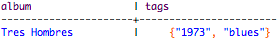
KEY to filter by key. This example features a collection of tags in the
playlists table. The query can index the tags, then filter on
'blues' in the tag set.
SELECT album, tags
FROM playlists
WHERE tags CONTAINS 'blues';
SELECT *
FROM playlists
WHERE venue CONTAINS 'The Fillmore';
SELECT *
FROM playlists
WHERE venue CONTAINS KEY '2014-09-22 22:00:00-0700';
Filtering a map's entries
CREATE INDEX blist_idx
ON cycling.birthday_list (ENTRIES(blist));
SELECT *
FROM cycling.birthday_list
WHERE blist['age'] = '23';
Filtering a full frozen collection
FROZEN collection (set, list, or map). The query retrieves rows that
fully match the collection's values.
CREATE INDEX rnumbers_idx
ON cycling.race_starts (FULL(rnumbers));
SELECT *
FROM cycling.race_starts
WHERE rnumbers = [39, 7, 14];
Range relations
DataStax Enterprise supports greater-than and less-than comparisons, but for a given partition key, the conditions on the clustering column are restricted to the filters that allow selection of a contiguous set of rows.
CREATE TABLE ruling_stewards (
  steward_name text,
  king text,
  reign_start int,
  event text,
  PRIMARY KEY (steward_name, king, reign_start)
);
king were not a component of the primary key, you
would need to create an index on king to use this
query:SELECT * FROM ruling_stewards WHERE king = 'Brego' AND reign_start >= 2450 AND reign_start < 2500 ALLOW FILTERING;
 steward_name | king  | reign_start | event
--------------+-------+-------------+--------------------
      Boromir | Brego |        2477 |   Attacks continue
       Cirion | Brego |        2489 | Defeat of Balchoth

(2 rows)
To
allow selection of a contiguous set of rows, the WHERE clause must
apply an equality condition to the king component of the primary key. The
ALLOW FILTERING clause is also required.
ALLOW FILTERING provides the capability to query the clustering columns
using any condition.
Only use ALLOW FILTERING for development. When you attempt a
potentially expensive query, such as searching a range of rows, DSE displays this
message:
Bad Request: Cannot execute this query as it might involve data
filtering and thus may have unpredictable performance. If you want
to execute this query despite the performance unpredictability,
use ALLOW FILTERING.
To run this type of query, use ALLOW FILTERING, and restrict the
output to n rows using LIMIT n. For example:
SELECT *
FROM ruling_stewards
WHERE king = 'none'
  AND reign_start >= 1500
  AND reign_start < 3000
LIMIT 10
ALLOW FILTERING;
Using LIMIT does not prevent all problems caused by ALLOW
FILTERING. In this example, if there are no entries without a value for
king, the SELECT scans the entire table, no
matter what the LIMIT is.
It is not necessary to use LIMIT with ALLOW
FILTERING, and LIMIT can be used by itself. But
LIMIT can prevent a query from ranging over all partitions in a
datacenter, or across multiple datacenters.
Using compound primary keys and sorting results
These restrictions apply when using anORDER BY clause with a compound primary
key: - Only include clustering columns in the
ORDER BYclause. - In the
WHEREclause, provide all the partition key values and clustering column values that precede the column(s) in theORDER BYclause. In 6.0 and later, the columns specified in theORDER BYclause must be an ordered subset of the columns of the clustering key; however, columns restricted by the equals operator (=) or a single-valuedINrestriction can be skipped. - When sorting multiple columns, the columns must be listed in the same order in the
ORDER BYclause as they are listed in thePRIMARY KEYclause of the table definition. - Sort ordering is limited. For example, if your table definition uses
CLUSTERING ORDER BY (start_month ASC, start_day ASC), then you can useORDER BY start_day, racein your query (ASCis the default). You can also reverse the sort ordering if you apply it to all of the columns; for example,ORDER BY start_day DESC, race DESC. - Refer to a column using the actual name, not an alias.
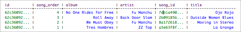
For example, set up the playlists table
(which uses a compound primary key), and use this query to get information about a
particular playlist, ordered by song_order. You do not need to include the ORDER
BY column in the select
expression.
SELECT *
FROM playlists
WHERE id = 62c36092-82a1-3a00-93d1-46196ee77204
ORDER BY song_order DESC
LIMIT 50;
Output:
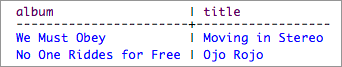
Or, create an index on playlist artists, and use this query to get titles of Fu Manchu songs on the playlist:
CREATE INDEX ON playlists(artist);
SELECT album, title
FROM playlists
WHERE artist = 'Fu Manchu';
Output:
Grouping results
The GROUP BY
clause condenses the selected rows that share the same values for a set of columns into a
group. A GROUP BY clause can contain:
- Partition key columns and clustering columns.
- A deterministic monotonic function, including a user-defined function (UDF), on the
last clustering column specified in the
GROUP BYclause. TheFLOOR()function is monotonic when the duration and start time parameters are constants. - A deterministic aggregate.
race_times_summary
table:CREATE TABLE cycling.race_times_summary ( race_date date, race_time time, PRIMARY KEY (race_date, race_time) );The table contains these rows:
 race_date  | race_time
------------+--------------------
 2019-03-21 | 10:01:18.000000000
 2019-03-21 | 10:15:20.000000000
 2019-03-21 | 11:15:38.000000000
 2019-03-21 | 12:15:40.000000000
 2018-07-26 | 10:01:18.000000000
 2018-07-26 | 10:15:20.000000000
 2018-07-26 | 11:15:38.000000000
 2018-07-26 | 12:15:40.000000000
 2017-04-14 | 10:01:18.000000000
 2017-04-14 | 10:15:20.000000000
 2017-04-14 | 11:15:38.000000000
 2017-04-14 | 12:15:40.000000000

(12 rows)race_date column
values:SELECT race_date, race_time FROM cycling.race_times_summary GROUP BY race_date;
race_date column value are grouped together
into one row in the query output. Three rows are returned because there are three groups
of rows with the same race_date column value. The value returned is the
first value that is found for the
group. race_date | race_time
------------+--------------------
2019-03-21 | 10:01:18.000000000
2018-07-26 | 10:01:18.000000000
2017-04-14 | 10:01:18.000000000
(3 rows)race_date and FLOOR(race_time,
1h), which returns the hour. The number of rows in each group is returned by
COUNT(*).SELECT race_date, FLOOR(race_time, 1h), COUNT(*) FROM cycling.race_times_summary GROUP BY race_date, FLOOR(race_time, 1h);Nine rows are returned because there are nine groups of rows with the same
race_date and FLOOR(race_time, 1h)
values: race_date | system.floor(race_time, 1h) | count
------------+-----------------------------+-------
2019-03-21 | 10:00:00.000000000 | 2
2019-03-21 | 11:00:00.000000000 | 1
2019-03-21 | 12:00:00.000000000 | 1
2018-07-26 | 10:00:00.000000000 | 2
2018-07-26 | 11:00:00.000000000 | 1
2018-07-26 | 12:00:00.000000000 | 1
2017-04-14 | 10:00:00.000000000 | 2
2017-04-14 | 11:00:00.000000000 | 1
2017-04-14 | 12:00:00.000000000 | 1
(9 rows)Computing aggregates
DSE provides standard built-in functions that return aggregate values to
SELECT statements.
Using COUNT() to get the non-null value count for a column
A SELECT expression using COUNT(column_name) returns
the number of non-null values in a column. COUNT ignores null values.
For example, count the number of last names in the cyclist_name
table:
SELECT COUNT(lastname)
FROM cycling.cyclist_name;
Getting the number of matching rows and aggregate values with COUNT()
A SELECT expression using COUNT(*) returns the number
of rows that matched the query. Use COUNT(1) to get the same result.
COUNT(*) or COUNT(1) can be used in conjunction with
other aggregate functions or columns.
This example counts the number of rows in the cyclist name table:
SELECT COUNT(*)
FROM cycling.cyclist_name;
This example calculates the maximum value for start day in the cycling events table and counts the number of rows returned:
SELECT start_month, MAX(start_day), COUNT(*)
FROM cycling.events
WHERE year = 2017
  AND discipline = 'Cyclo-cross';
This example provides a year that is not stored in the events table:
SELECT start_month, MAX(start_day)
FROM cycling.events
WHERE year = 2022
ALLOW FILTERING;
 start_month | system.max(start_day)
-------------+-----------------------
        null |                  null

(1 rows)
Getting maximum and minimum values in a column
SELECT expression using
MAX(column_name) returns the maximum value in a
column. When the column's data type is numeric (bigint,
decimal, double, float,
int, or smallint), this returns the maximum value.
SELECT MAX(race_points)
FROM cycling.cyclist_points
WHERE id = e3b19ec4-774a-4d1c-9e5a-decec1e30aac;
 system.max(race_points)
-------------------------
120WHERE clause, a warning message is displayed:
Warnings :
Aggregation query used without partition keyMIN function returns the minimum
value:SELECT MIN(race_points) FROM cycling.cyclist_points WHERE id = e3b19ec4-774a-4d1c-9e5a-decec1e30aac;
 system.min(race_points)
-------------------------
                       6
If the column referenced by MAX or MIN has an
ascii or text data type, these functions return the
last or first item in an alphabetic sort of the column values. If the specified column has
data type date or timestamp, these functions return the
most recent or least recent times and dates. If a column has a null value,
MAX and MIN ignores that value; if the column for an
entire set of rows contains null, MAX and MIN return
null.
If the query includes a WHERE clause (recommended), MAX
or MIN returns the largest or smallest value from the rows that satisfy
the WHERE condition.
Getting the average or sum of a column of numbers
DSE computes the average of all values in a column when AVG is used in
the SELECT statement:
SELECT AVG(race_points)
FROM cycling.cyclist_points
WHERE id = e3b19ec4-774a-4d1c-9e5a-decec1e30aac;
 system.avg(race_points)
-------------------------
                      67
Using SUM to get a total:
SELECT SUM(race_points)
FROM cycling.cyclist_points
WHERE id = e3b19ec4-774a-4d1c-9e5a-decec1e30aac; system.sum(race_points)
-------------------------
201
(1 rows)If any of the rows returned have a null value for the column referenced for a
SUM or AVG aggregation function, the function includes
that row in the row count, but uses a zero value to calculate the average. The
SUM and AVG functions do not work with
text, uuid, or date fields.
Retrieving the date/time a write occurred
The WRITETIME function applied to a column returns the date/time in microseconds at which the column was written to the database.
For example, to retrieve the date/time that writes occurred to the firstname column of a cyclist:
SELECT WRITETIME (firstname)
FROM cycling.cyclist_points
WHERE id = e3b19ec4-774a-4d1c-9e5a-decec1e30aac;
 writetime(firstname)
----------------------
     1538688876521481
     1538688876523973
     1538688876525239
The WRITETIME output of the last write 1538688876525239
in microseconds converts to Thursday, October 4, 2018 4:34:36.525 PM GMT-05:00
DST.
Retrieving the time-to-live of a column
INSERT INTO cycling.calendar (
  race_id, race_name, race_start_date, race_end_date
) VALUES (
  200, 'placeholder', '2015-05-27', '2015-05-27'
)
USING TTL 100;
UPDATE cycling.calendar
USING TTL 300
SET race_name = 'dummy'
WHERE race_id = 200
  AND race_start_date = '2015-05-27'
  AND race_end_date = '2015-05-27';
After inserting the TTL, use SELECT statement to check its current value:
SELECT TTL(race_name)
FROM cycling.calendar
WHERE race_id = 200;
Output:
 ttl(race_name)
----------------
            276

(1 rows)
Retrieving values in the JSON format
For details, see Retrieval using JSON