Schema configuration tuning

Disclaimer

This document provides general recommendations for DataStax Enterprise (DSE) and Apache Cassandra™. This document requires either basic DSE or Cassandra knowledge, or both. This document does not replace the official documentation.

As described in Data model and schema configuration checks, data modeling is a critical part of a project’s success. Additionally, the performance of the Cassandra or DSE cluster is influenced by schema configuration. Cassandra and DataStax Enterprise allow you to specify per-table configuration parameters, such as compaction strategy, compression of data, and more. This document describes the configuration parameters that are often changed, and provides advice on their tuning when it is applicable.

Compaction strategy

Before taking a deep dive on compaction algorithms, let us review how data is written to disk:

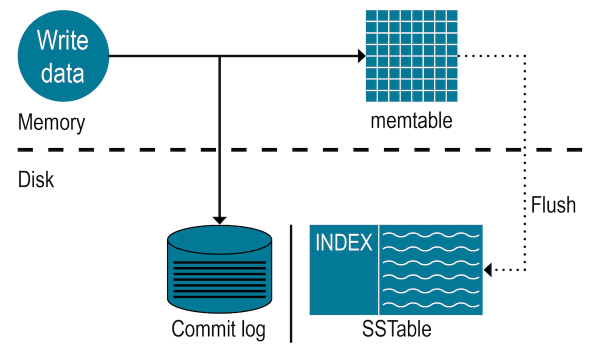
As this image shows, Cassandra processes data at several stages on the write path, starting with the immediate logging of a write and ending with writing data to disk:

Logs data in the commit log.
Writes data to the memtable.
Flushes data from the memtable, which is condition-based and set by configuration parameters in the cassandra.yaml file. The location of this file depends on the type of installation:
- Package installations: /etc/dse/cassandra/cassandra.yaml
- Tarball installations: <installation_location>/resources/cassandra/conf/cassandra.yaml
Stores data on disk in SSTables.

SSTables are immutable. The data contained in them are never updated or deleted in place. Instead, when a new write is performed, changes are written to a new memtable and then a new SSTable.

A compaction process runs in the background that merges SSTables together. Otherwise, the more SSTables touched on the read path, the higher the latencies become. Ideally, when the database is properly tuned, a single query does not touch more than two or three SSTables.

DSE provides a few main compaction strategies, each for a specific use case:

UCS: Utilizes and improves upon STCS or LTC, and is a hybrid mix of the two. It is good for a mixed workload of reads and writes.
STCS: Good for write-heavy cases.
LCS: Good for read-heavy use cases. This strategy reduces the spread of data across multiple SSTables.
TWCS: Good for time series or for any table with TTL (Time-to-live).

Before reviewing the compaction parameters that tune SSTables, here are some pros and cons for each compaction strategy:

Compaction

Pros

Cons

UCS (DSE 6.8.25+)

Useful for any workload. Unifies and improves tiered (STCS) and leveled (LCS) compaction strategies. Utilizes sharding (partitioned data compacted in parallel). Provides configurable read, write amplification guarantees. Parameters are reconfigurable at any time. UCS reduces disk space overhead and is stateless.

Consider using UCS if your legacy compaction strategy is not optimum.

UCS behavior is not meant to mirror TWCS’s append-only time series data compaction.

STCS

Provides more compaction throughput and more aggressive compaction compared to LCS. In some read-heavy use cases, if data is overly spread, it is better to have a more aggressive compaction strategy.

Requires leaving 50% free disk space to allow for compaction or four times the largest SSTable file on disk (two copies + new file).

SSTable files can grow to very large files that can stay on disk for a long time.

Inconsistent performance because data are spread across many SSTables files. When data are frequently updated, single rows can spread across multiple SSTables and impact system performance.

LCS

Reduces the number of SSTable files that are touched on the read path since there is no overlap for a single partition (single SSTable) above level 0.

Reduces s free space needed for compaction.

Recommended node density is 500GB, which is fairly low. Limited number (2) of potential compactors due to internal algorithms that require locking.

Write amplification consumes more IO.

TWCS

Provides capability to increase node densities. TTL data does not stress the system with tombstones because SSTables get dropped in a single action.

If not initially used, reloading data with a proper windowing layout is not possible.

Common compaction configuration parameters

If you see a lot of pending compactions, the system probably requires tuning. The two main parameters for compaction are:

concurrent_compactors: The number of parallel threads performing compaction.

Start to increase the compaction_throughput_mb_per_sec before and only change this value if you have enough IO. STCS and TWCS benefit if this value is increased, but LCS does not use more than 2 compactors at any time.
compaction_throughput_mb_per_sec: The throughput in MB/s for the compactor process. This is a limit for all compaction threads together, not per thread!

Consider that as more compactions are performed, the more resources are consumed and the Garbage Collector (GC) pressure is increased.

To retrieve pending compactions, use your preferred monitoring solution or one of the following commands:

nodetool sjk mx -f Value -mg -b org.apache.cassandra.metrics:type=Compaction,name=PendingTasks

nodetool compactionstats

Be aware that tombstones can trigger compaction outside of the compaction strategy due on the following configuration parameters:

tombstone_compaction_interval: A single-SSTable compaction is triggered based on the estimated tombstone ratio. This option makes the minimum interval between two single-SSTable compactions tunable.

Default: 1 day.
unchecked_tombstone_compaction: A single-SSTable compaction every day (default tombstone_compaction_interval), as long as the estimated tombstone ratio is higher than tombstone_threshold. In order to evict tombstones faster, you can reduce this value, but the system consumes more resources.
tombstone_threshold: The ratio of garbage-collectable (GC) tombstones to all contained columns.

The following sections contain the list of parameters available by compaction type. Only change these parameters if you have not been able to improve the compaction performance with the above configuration parameters.

Unified Compaction Strategy (UCS)

This compaction strategy is highly versatile and useful with any size workload. It unifies and improves upon tiered (STCS) and leveled (LCS) compaction strategies, adds sharding (subsetting SSTables), and is reconfigurable at any time.

UCS groups SSTables in levels based on the logarithm of the SSTable size, with a fanout (F) factor as the base of the logarithm and with each level triggering a compaction as soon as it has T SSTables. The set F and T parameters and minimum SSTable size determine UCS behavior. UCS combines the two parameters into one integer W value. These values are set accordingly:

If W < 0, then F = 2 - W and T = 2. This means leveled compactions with high WA, but low RA.
If W > 0, then set F = 2 + W and T = F. This means tiered compactions with low WA, but high RA.
If W = 0, then F = T = 2. This is the middle ground, with leveled and tiered compactions behave identically.

Because levels can be set to different values of W, levels can behave differently. For example, level zero (0) could behave like STCS but higher levels could increasingly behave like LCS.

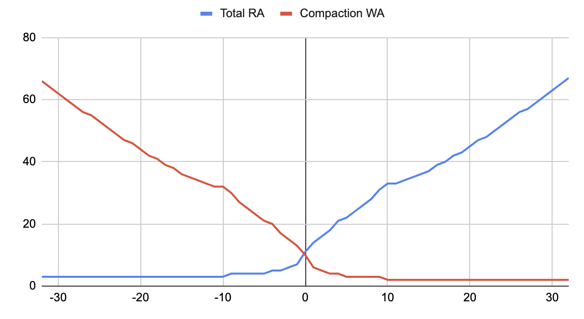
Unified compaction with varying `W` values

This image depicts varying read amplifications (RA) and write amplifications (WA) given different W factor values. STCS-like behavior favors write-heavy workloads, while LCS-like behavior is good for ready-heavy workloads.

The UCS strategy also introduces compaction shards. Data is partitioned in independent shards that can be compacted in parallel. Shards are defined by splitting the token ranges for which the node is responsible into equally-sized sections.

Several parameters are available for tuning UCS compaction:

static_scaling_factors: An integer value specifying W for all levels of the hierarchy. Positive values specify tiered compaction, and negative values specify leveled, with fan factor |W|+2. Increasing W improves write amplification at the expense of reads, and decreasing it improves reads at the expense of writes.

Default: 2, which is similar to using STCS with its default threshold of 4.

A value of -8 uses the equivalent of LCS with its default fan factor of 10.

The option also accepts a comma separated value list of integers, in which case different values may be passed for the levels of the hierarchy. The first value sets the value of W for the first level, the second value for the second level, and so on. The last value in this list is also used for all remaining levels that are otherwise unspecified.

To increase the probability for compaction, you can reduce this value. However, as more compactions are triggered, the more resources are consumed.
num_shards: This is the number of shards. It is recommended that users set this value. More shards means more parallelism and smaller SSTables at the higher levels at the expense of somewhat higher CPU usage.

Default: 10 * disks. This is the number of disk volumes defined in the cassandra.yaml configuration file.

For example, if there are 5 disks, there would be 50 shards. With a data size of 10 TB, the shard size would be 200 GB, which is an upper bound for the size of the largest SSTables and compaction operations.
min_sstable_size_in_mb: This is the minimum SSTable size in MB under which data is not split on shard boundaries. Higher values mean fewer SSTables on disk and larger compaction operations on the lowest levels of the hierarchy. Storage-attached secondary indexes work better with higher minimum SSTable sizes.

Default: 100.
dataset_size_in_gb: This parameter is the target dataset size, by default the minimum total space for all the data file directories. It calculates the number of levels and therefore the theoretical read and write amplification. Accuracy is not crucial, but it is recommended that the parameter is set to a value within a few GBs of the target local dataset size. If not specified, the database uses the total space on the devices containing the data directories, and assuming that data is equally split among them.
max_space_overhead: The maximum permitted space overhead as a fraction of the dataset size. This parameter cannot be smaller than 1/num_shards, as that value limits the extra space that is required to complete compactions. UCS only runs compactions that do not exceed this limit. For example, for a dataset size of 10TB and 20% max overhead, if a 1.1TB compaction is currently running, UCS only starts the 1.1TB one in the next shard after it completes. UCS never starts compactions that are larger than the limit by themselves, so that the process will not run out of space. A warning is issued if the compaction is not started, as it may cause performance to deteriorate.

Default: 0.2 (20%).
expired_sstable_check_frequency_seconds: Determines how often to check for expired SSTables.

Default: 10 minutes.
unsafe_aggressive_sstable_expiration: Expired SSTables are dropped without checking if their data is shadowing other SSTables. This flag can only be enabled if cassandra.allow_unsafe_aggressive_sstable_expiration is true. Turning this flag can cause correctness issues, such as the re-appearing of deleted data. See discussions in CASSANDRA-13418, and DB-902 in Apache Software Foundation (ASF) Jira for valid use cases and potential problems.

Default: false

A recommended starting point uses the following, setting log_all to true for testing purposes:

compaction = "{'class': 'UnifiedCompactionStrategy',
                    'static_scaling_factors':'2',
                    'log_all':'true'}";

To upgrade SSTables that currently use STCS, use the following:

compaction = "{'class': 'UnifiedCompactionStrategy',
                    'static_scaling_factors':'2',
                    'log_all':'true'}";

To upgrade SSTables that currently use LCS, use the following:

compaction = "{'class': 'UnifiedCompactionStrategy',
                    'static_scaling_factors':'-2',
                    'log_all':'true'}";

Upgrading a UCS compaction strategy applies to newly created SSTables. Use nodetool upgradesstables -a <keyspace table> to apply UCS compaction settings to existing DSE SSTables.

In the cassandra.yaml configuration file, set the concurrent_compactors parameter to indicate the number of compaction threads available. Set this parameter to a large number, at minimum the number of expected levels of the compaction hierarchy to make sure that each level is given a dedicated compaction thread. The parameter avoids latency spikes, caused by lower levels of the compaction hierarchy not getting a chance to run.

Size Tiered Compaction Strategy (STCS)

With this compaction strategy, after the database sees enough tables of similar size in the range [average_sze * bucket_low, average_sze * bucket_high], the compaction merges the SSTables into a single file. As shown below, the files continue to increase in size as time passes:

Size tiered compaction after many inserts

Several parameters are available for tuning STCS compaction, but generally only two are required and only for special cases:

min_threshold: The minimum number of SSTables required to trigger a minor compaction.

To increase the probability for compaction, you can reduce this value. However, as more compactions are triggered, the more resources are consumed.
min_sstable_size: STCS groups SSTables into buckets.

The bucketing process groups SSTables that differ in size by less than 50%. The bucketing process is too fine-grained for small SSTables. If your SSTables are small, use min_sstable_size to define a size threshold (in bytes), below which all SSTables belong to one unique bucket. The best practice is to limit the number of SSTables for a single table between 15 and 25. If you see a number higher than 25, update the configuration to compact more often.

Leveled Compaction Strategy (LCS)

The leveled compaction strategy creates SSTables of a fixed, relatively small size (default is 160 MB) that are grouped into levels. Within each level, SSTables are guaranteed to be non-overlapping. Below shows a simple representation of the movement of data across the levels:

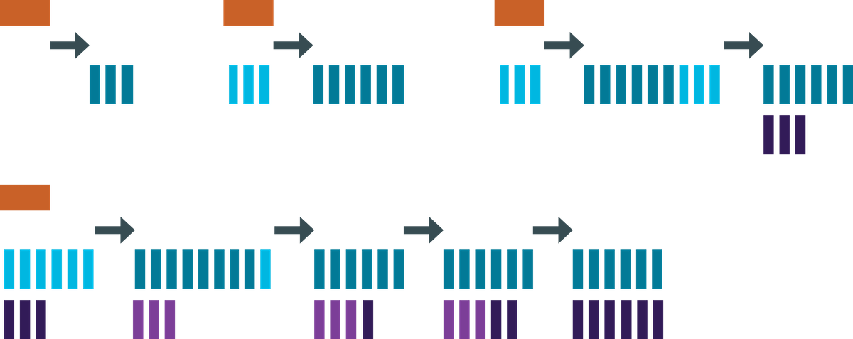
Configurable parameters for LCS include sstable_size_in_mb, which sets the target size for SSTables.

For very large partitions, the LCS compaction algorithm does not split data into multiple SSTables. This guarantees a single SSTable per level condition.

Because L0 can be a chaos space, be careful to properly tune all memtable parameters as well. In read-heavy use cases, DataStax recommends flushing memtables less frequently than when using STCS compaction.

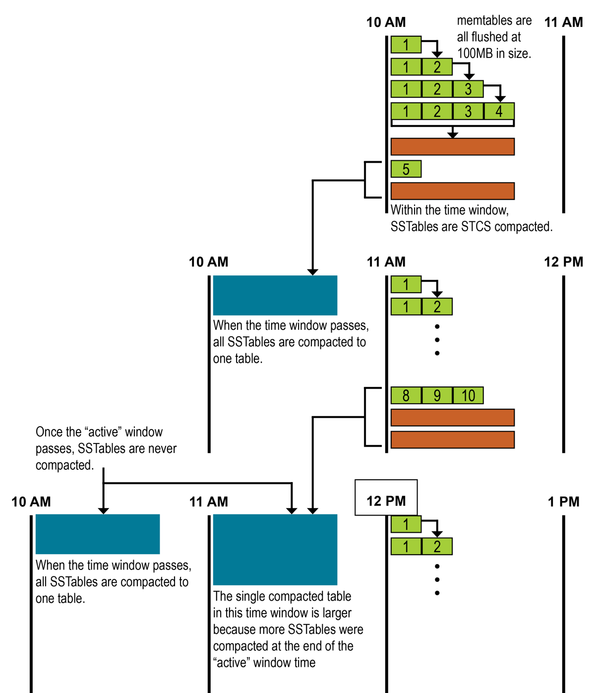
Time Window Compaction Strategy

This compaction strategy supersedes DTCS starting with Cassandra 3.0. It is perfect for all time series use cases or scenarios where data is assigned a Time-to-live (TTL) period. The main principle is to bucketize the time horizon by defining a window of compaction where only the current active window compacts using the STCS algorithm. Once a window is completed, the database compacts all files allocated for the bucket into a single file. Within the active window the system behaves as STCS and all STCS parameters are applicable.

In addition to the STCS configuration parameters, the TWCS has the following parameters:

compaction_window_unit: Time unit for defining the window size (milliseconds, seconds, hours, and so on).
compaction_window_size: Number of units per window (1, 2, 3, and so on).

Because the first bucket uses the STCS strategy, keep the total number of SSTable files around 20 for optimal compaction performance. In addition, limit the total number of inactive windows to below 30 (maximum 50).

Your use case might justify different values. To ensure performance does not degrade over time, be sure to properly test at scale.

To illustrate a time series use case:

Imagine an iOT use case with a requirement to retain data for a period of 1 year (TTL = 365 days). Looking at the prior recommendations, the window size should be equal to 365/30 ⇒ ~ 12 days with unit DAYS. With this configuration, only the data received during the last 12 days is compacted and everything else stays immutable, thus reducing the compaction overhead on the system.

Compression

To decrease the disk consumption, by default Cassandra stores data on the disk in compressed form. However, incorrectly configured compression may significantly harm the performance, so it makes sense to use correct settings. Existing settings can be obtained by executing the DESCRIBE TABLE command and looking for the compression parameter.

To change settings, use:

ALTER TABLE <name> WITH compression = {…}

If you change the compression settings, be aware that they apply only to newly created SSTables. If you want to apply them to existing data, use:

nodetool upgradesstables -a keyspace table.

For more information about internals of compression in Cassandra, see Performance Tuning - Compression with Mixed Workloads.

Compression algorithm

By default, tables on disk are compressed using the LZ4 compression algorithm. This algorithm provides a good balance between compression efficiency and additional CPU load arising from the use of compression.

Cassandra also supports other compression schemas (set via sstable_compression field of compression parameter):

Snappy (SnappyCompressor): Uses a compression ratio similar to LZ4, but it is much slower. It was used by default in the earlier versions of Cassandra, and if it is still used, DataStax recommends switching to LZ4.

Cassandra 4.0 has experimental support for the Zstandard compression algorithm.

Deflate (DeflateCompressor): Provides a better compression ratio than other compression algorithms, but it generates much more CPU load and is much slower. Use it only after careful testing.
None (empty string): Disables compression completely. It’s useful for removing overhead from decompression of data during read operations, especially for tables with small rows.
Compressed block size: By default, the chunk size of compressed data is 64Kb. This means that the database needs to read the entire amount to extract the necessary data and puts an additional load on the disk system when not needed. You can tune the chunk size to use lower values, like 16Kb or 32Kb. The Performance Tuning - Compression with Mixed Workloads blog shows the effects of using smaller compression chunk sizes using the value of the chunk_length_kb attribute of the table.

Be sure to take into account that reducing the chunk length can increase the amount of data stored on disk as the efficiency of compression decreases.

Decreasing chunk size should be done only for tables that have random access to data stored in tables.

Read repair chance

Cassandra has two types of read repair:

foreground: Repair happens when Cassandra detects data inconsistency during the read operation and blocks application operations until the repair process is complete.
background: Done proactively for a percentage of read operations. (Does not apply to all versions.)

The read_repair_chance and dclocal_read_repair_chance settings control the probability that background read repair will be performed in the whole cluster or only in the local datacenter. Unfortunately this implementation does not always work as designed; there are even bugs when local read repair in the current datacenter that can lead to the cross-datacenter operations, which can impact system performance (CASSANDRA-9753). In cases of the data inconsistency, when the read operations are performed with LOCAL_QUORUM or QUORUM consistency levels, the foreground read repair happens anyway (inside local datacenter, or in the whole cluster). This means that triggering the additional repairs is unnecessary.

To disable background read repair, set both settings to 0. If you are using a Cassandra or DSE version where this functionality still exists, see CASSANDRA-13910. To disable background read repair, use the following script on one of the nodes:

Bloom filter tuning

Bloom filter is an internal data structure that optimizes reading of the data from the disk. It is created for every SSTable file in the system and is loaded into the off-heap memory. The size of memory consumed is proportional to the number of partition keys stored in the specific SSTable. In some cases it can be significant, up to tens of gigabytes.

To check the amount of memory allocated to bloom filters per table, execute nodetool tablestats (or nodetool cfstats on older Cassandra versions ), and check the number in the line Bloom filter off heap memory used, which displays the size of bloom filter in bytes.

You can control the size of the bloom filter by tuning the bloom_filter_fp_chance option on a specific table. This parameter increases the false positive ratio, so the bloom filter is smaller. For example, increasing the false positive ratio to 10% can decrease memory consumption for bloom filter by almost two times. (See Bloom Filter Calculator) However, an increased false positive ratio can cause more SSTables to be read than is necessary. Tuning bloom filters should be done only for tables that have rarely-accessed data, such as an archive where data are stored only for compliance and are rarely read or read by batch jobs.

Garbage collection of tombstones

Cassandra does not delete data directly, but uses a special marker called tombstone. A tombstone shadows the deleted data. For details, see About Deletes and Tombstones in Cassandra. A tombstone is stored in the files for at least the period of time defined by the configuration parameter gc_grace_seconds. The default is 10 days (864000 seconds). Keep in mind that if one or more nodes in a cluster were down during the deletion of the data, those nodes must be returned to the cluster and repair performed during this period of time; otherwise deleted data could be resurrected. If a server was down longer than this period, then remove all Cassandra data from it and perform a node replacement.

Starting with DSE 6.0, Nodesync prevents removal of the tombstones on tables that have Nodesync enabled until Cassandra makes sure that tombstones are synchronized to all replicas. If Nodesync is slow and cannot synchronize data fast enough, it may lead to an increase in the number of tombstones contained in tables for a significant amount of time.

A significant number of tombstones in the table can negatively impact the performance of the read operations, and in some cases you may need to decrease the value of the gc_grace_seconds parameter to remove tombstones faster. If this value is changed, you need to ensure that the full token range repair is performed during the specified period of time. Doing this can be challenging if node was down for a significant amount of time.

Also, a too low value in gc_grace_seconds can impact hinted handoff by preventing collection and by replaying hints. In this case, it requires data repair.

Caching

Caching of data, actual or auxiliary, influences the read performance of the Cassandra and DSE nodes (see How is data read?). For tables you can tune two things specified in the caching configuration parameter:

Caching of the partition keys (the keys argument, possible values are ALL and NONE). This cache keeps the mapping of the partition key value into the compression offset map that identifies the compressed block on disk containing the data. If the partition key exists in the key cache, Cassandra may skip some steps when reading the data and subsequently increase read performance. The size of the key cache for all tables is specified in the cassandra.yaml file, and you should use nodetool info to check its efficiency. If cache is full and the hit ratio is below 90%, it could signal that you should increase the size of the key cache.

Starting with DSE 6, a new SSTable file format is introduced that does not require caching of the partition keys. As a result, this feature is only useful for files in old formats.

Caching of the individual rows per partition (the rows_per_partition argument, possible values are ALL, NONE, or a numeric value). Caching frequently used rows can speed up data access because the data is stored in memory. Generally use it for mostly-read workloads as changing the rows and partitions invalidates the corresponding entries in the cache and requires re-population of the cache (by reading from the disk).

By default, Cassandra has the following configuration (cache all partition keys and do not cache rows):

caching = {'keys': 'ALL', 'rows_per_partition': 'NONE'}

If needed, you can change it with the ALTER TABLE command (to allow caching of all partition keys, and 10 rows per partition):

ALTER TABLE ks.tbl WITH caching = {'keys': 'ALL', 'rows_per_partition': 10};

Speculative Retry

By default, a coordinator node sends queries to as many replicas as necessary to satisfy consistency levels: one for consistency level ONE, a quorum for QUORUM, and so on. Using the configuration parameter speculative_retry, you can specify when coordinators may query additional replicas. This is useful when replicas to which queries were sent by coordinator are slow or unresponsive. Speculative retries are used to reduce the 95 or 99 percentiles tail read latencies, but they put more load on the Cassandra nodes, which may need to handle more read requests than necessary. Keep the default value of 99PERCENTILE until you become familiar with the process.

The speculative_retry setting does not effect reads with consistency level ALL because they already query all replicas.

This speculative_retry configuration parameter has the following values (case-insensitive):

ALWAYS: The coordinator node sends extra read requests to all other replicas for every read of that table.
Xpercentile: The read latency of each table is tracked, and coordinator node calculates X percentile of the typical read latency for a given table. The coordinator sends additional read requests once the wait time exceeds the calculated time. The problem with this setting is that when a node is unavailable, it increases the read latencies and as result increases the calculated values.
Nms: The coordinator node sends extra read requests to all other replicas when the coordinator node has not received responses within N milliseconds.
NONE: The coordinator node does not send additional read requests.

In Cassandra 4.0, speculative_retry may have additional values. See CASSANDRA-13876 and CASSANDRA-14293.

Memtable flushing

Usually, Cassandra flushes memtable data to disk in the following situations:

The memtable flush threshold is met.
On shutdown.
When either nodetool flush or nodetool drain is executed.
When commit logs get full.

It is also possible to explicitly flush data from a memtable on the regular cadence. This is regulated by the memtable_flush_period_in_ms configuration parameter. Usually, this parameter is best left with its default value (zero) so memtables are flushed as previously described. Tune this parameter only in rare situations and only for specific tables. An example is a table with very rare modifications that does not need commit logs sitting on the disk for a long period of time. In this case, set this parameter to flush memtable of a given table to every day, or every X hours.

This parameter is in the milliseconds!