SELECT
Queries data in one table. The results are returned as a set of rows.
There are several selectors, clauses, functions, and options you can use to refine queries:
|
A You can use TRACING to analyze the impact of various queries in your environment.
|
Partition keys
A query requires that all partitions are restricted, except when querying with an index. Use logical operators in query statements to identify the partition key columns:
-
Equals (
=): Any partition key column. -
IN: Restricted to the last column of the partition key or the last column of the full primary key when searching multiple partitions. -
Range (
>=,⇐,>, and<) on tokens: Fully tokenized partition key where all partition key columns are specified in order (as set in the table definition) as arguments of theTOKENfunction. Use token ranges to scan data stored on a particular node.
For more information about these operators, see WHERE clause.
Synopsis
SELECT [ JSON | DISTINCT ] <selectors>
  FROM [<keyspace_name>.]<table_name>
  [ WHERE [ <primary_key_conditions> | <non_primary_key_conditions> IN (<column_name> [, ...]) ALLOW FILTERING ] [ AND ] [ <index_conditions> ] ]
  [ GROUP BY <column_name> [ , ... ] ]
  [ ORDER BY <column_name> ( ASC | DESC ) [ , ... ] ] |
  [ ORDER BY <vector_column_name> ANN OF [n,n,n,...] [ LIMIT N ] ]
  [ ( LIMIT <N> [ OFFSET <N> ]  | PER PARTITION LIMIT <N> ) ]
[ ALLOW FILTERING ] ;| Syntax conventions | Description |
|---|---|
UPPERCASE |
Literal keyword. |
Lowercase |
Not literal. |
|
Variable value. Replace with a user-defined value. |
|
Optional.
Square brackets ( |
|
Group.
Parentheses ( |
|
Or.
A vertical bar ( |
|
Repeatable.
An ellipsis ( |
|
Single quotation ( |
|
Map collection.
Braces ( |
|
Set, list, map, or tuple.
Angle brackets ( |
|
End CQL statement.
A semicolon ( |
|
Separate the command line options from the command arguments with two hyphens ( |
|
Search CQL only: Single quotation marks ( |
|
Search CQL only: Identify the entity and literal value to overwrite the XML element in the schema and solrConfig files. |
Parameters
| Parameter | Description | Default |
|---|---|---|
|
Optional. Name of the keyspace that contains the table to select. |
If no name is specified, the current keyspace is used. |
|
Name of the table to select. |
|
|
Name of the column to select. |
|
|
Name of the vector column to select. |
Selectors
The SELECT statement is used to query data from a table in CQL.
The results are returned as a set of rows.
Selectors are used to specify which columns are queried and returned.
The SELECT statement can also transform the data on return using functions.
Table data also has related metadata that can be returned using metadata functions.
Return all columns
To return all columns from a table, use the wildcard * selector.
SELECT * FROM cycling.cyclist_name; id | firstname | lastname
--------------------------------------+-----------+-----------------
e7ae5cf3-d358-4d99-b900-85902fda9bb0 | Alex | FRAME
fb372533-eb95-4bb4-8685-6ef61e994caa | Michael | MATTHEWS
5b6962dd-3f90-4c93-8f61-eabfa4a803e2 | Marianne | VOS
220844bf-4860-49d6-9a4b-6b5d3a79cbfb | Paolo | TIRALONGO
6ab09bec-e68e-48d9-a5f8-97e6fb4c9b47 | Steven | KRUIKSWIJK
e7cd5752-bc0d-4157-a80f-7523add8dbcd | Anna | VAN DER BREGGEN
(6 rows)Since the * selector returns all columns, it is not necessary to specify the column names.
The more columns a table has, the more resources are required to return the data.
Return specific columns
Because the number of columns returned can affect performance, it is recommended to specify the columns to return, if possible.
For example, to return only the lastname column from the cycling.cyclist_name table:
SELECT lastname FROM cycling.cyclist_name; lastname
-----------------
FRAME
MATTHEWS
VOS
TIRALONGO
KRUIKSWIJK
VAN DER BREGGEN
(6 rows)To return multiple columns, separate the column names with a comma:
SELECT lastname, firstname FROM cycling.cyclist_name; lastname | firstname
-----------------+-----------
FRAME | Alex
MATTHEWS | Michael
VOS | Marianne
TIRALONGO | Paolo
KRUIKSWIJK | Steven
VAN DER BREGGEN | Anna
(6 rows)Columns can be renamed on return using an alias:
SELECT id, cyclist_age AS age FROM cycling.cyclist_alt_stats LIMIT 3; id | age
--------------------------------------+------
e0953617-07eb-4c82-8f91-3b2757981625 | null
1ba0417d-62da-4103-b710-de6fb222db6f | 34
4ceb495c-55ab-4f71-83b9-81117252bf13 | 34
(3 rows)|
A column alias cannot be used in the |
Return transformed data
The SELECT statement can transform the data on return using functions.
The functions are varied and can be used to manipulate the data in different ways.
For example, JSON can be used to return all columns as JSON, toJson to return selected column as JSON, or CAST can be used to change the data type of a column.
Distinct column values can be returned using the DISTINCT function.
The number of rows with a particular column can be returned using the COUNT function.
Any native or user-defined functions can be used to transform the data, such as the SUM or AVG function.
Any user-defined aggregate function can be used to transform the data, such as the average function.
The TOKEN function can be used to return the token value of a column.
To output selected data from a table in JSON format, use the JSON function:
SELECT JSON * FROM cycling.birthday_list; [json]
----------------------------------------------------------------------------------------------------------
{"cyclist_name": "Claudio HEINEN", "blist": {"age": "23", "bday": "27/07/1992", "nation": "GERMANY"}}
{"cyclist_name": "Claudio VANDELLI", "blist": {"age": "54", "bday": "27/07/1961", "nation": "ITALY"}}
{"cyclist_name": "Luc HAGENAARS", "blist": {"age": "28", "bday": "27/07/1987", "nation": "NETHERLANDS"}}
{"cyclist_name": "Toine POELS", "blist": {"age": "52", "bday": "27/07/1963", "nation": "NETHERLANDS"}}
{"cyclist_name": "Allan DAVIS", "blist": {"age": "35", "bday": "27/07/1980", "nation": "AUSTRALIA"}}
{"cyclist_name": "Laurence BOURQUE", "blist": {"age": "23", "bday": "27/07/1992", "nation": "CANADA"}}
(6 rows)Note the nested JSON structure in the output, with the column name as the key and the column value as the value.
To specify the JSON format for a particular column, enclose its name in the toJson() function.
A JSON-formatted timestamp column can include complete time zone information.
SELECT id, commenter, toJson(created_at) FROM cycling.comments_vs; id | commenter | system.tojson(created_at)
--------------------------------------+-----------+----------------------------
e8ae5cf3-d358-4d99-b900-85902fda9bb0 | John | "2017-04-01 14:33:02.160Z"
e7ae5cf3-d358-4d99-b900-85902fda9bb0 | Alex | "2017-04-01 14:33:02.160Z"
e7ae5cf3-d358-4d99-b900-85902fda9bb0 | Alex | "2017-03-21 21:11:09.999Z"
e7ae5cf3-d358-4d99-b900-85902fda9bb0 | Alex | "2017-02-14 20:43:20.000Z"
c7fceba0-c141-4207-9494-a29f9809de6f | Amy | "2024-06-07 03:04:35.620Z"
c7fceba0-c141-4207-9494-a29f9809de6f | Amy | "2017-04-01 13:43:08.030Z"
c7fceba0-c141-4207-9494-a29f9809de6f | Amy | "2017-03-22 01:16:59.001Z"
c7fceba0-c141-4207-9494-a29f9809de6f | Amy | "2017-02-17 08:43:20.234Z"
c7fceba0-c141-3207-9494-a29f9809de6f | Amy | "2017-02-17 08:43:20.234Z"
c7fceba0-c141-7207-9494-a29f9809de6f | Amy | "2024-06-07 03:04:35.624Z"
e8ae5df3-d358-4d99-b900-85902fda9bb0 | Jane | "2017-04-01 14:33:02.160Z"
c7fceba0-c141-4207-9594-a29f9809de6f | Jane | "2017-02-17 08:43:20.234Z"
(12 rows)To cast a column to a different data type, use the CAST function:
SELECT CAST(created_at AS date) FROM cycling.comments; cast(created_at as date)
--------------------------
2023-04-01
2024-06-07
(2 rows)If a table has duplicate values in a column, use the DISTINCT function to return only the unique values:
SELECT DISTINCT country FROM cycling.country_flag; country
---------
Belgium
France
(2 rows)To count the number of rows in a column, use the COUNT function:
SELECT start_month, MAX(start_day), COUNT(*) FROM cycling.events
  WHERE year = 2017 AND discipline = 'Cyclo-cross';
start_month | system.max(start_day) | count
-------------+-----------------------+-------
1 | 28 | 11
(1 rows)To use the COUNT function with a WHERE clause, include the COUNT function in the SELECT list and the WHERE clause in the query.
For example, to get the number of cyclists from Belgium:
SELECT count(cyclist_name) FROM cycling.country_flag
  WHERE country='Belgium';
system.count(cyclist_name)
----------------------------
2
(1 rows)A number of native functions can be used to transform the data.
The data is transformed only on return, rather than stored in the table.
These are general functions that are familiar to most people, such as the average, or AVG function:
SELECT AVG(race_points) FROM cycling.cyclist_points
  WHERE id = e3b19ec4-774a-4d1c-9e5a-decec1e30aac;
system.avg(race_points)
-------------------------
67
(1 rows)User-defined functions can also be used to transform the data:
SELECT left(firstname, 1), lastname FROM cycling.cyclist_name; cycling.left(firstname, 1) | lastname
----------------------------+-----------------
A | FRAME
null | MATTHEWS
null | VOS
P | TIRALONGO
M | VOS
S | KRUIKSWIJK
A | VAN DER BREGGEN
(7 rows)User-defined aggregates can also be used to transform the data.
For examples, the 'average` function can be used to retrieve the average of the column cyclist_time_sec from a table:
SELECT average(cyclist_time_sec) AS Average FROM cycling.team_average
  WHERE team_name = 'UnitedHealthCare Pro Cycling Womens Team';
average
-------------
11474.66667
(1 rows)
Warnings :
User defined function cycling.average_state : (tuple<int, bigint>, int) -> tuple<int, bigint> consumed more than 500µs CPU time (4183µs)The TOKEN function can be used to return the token value of a column.
The token value is the hashed value of the partition key, thus it can only be used on the partition key column or columns.
This function is useful when using the token value in a query to filter data with a WHERE clause.
To return the token value of the race_id column in the cycling.race table:
SELECT race_name AS name,race_year AS year FROM cycling.rank_by_year_and_name
  WHERE TOKEN(race_year,race_name) >= 4582455970709790046;
name | year
--------------------------------------------+------
Tour of Japan - Stage 4 - Minami > Shinshu | 2015
Tour of Japan - Stage 4 - Minami > Shinshu | 2015
Tour of Japan - Stage 4 - Minami > Shinshu | 2015
(3 rows)Return column metadata
Each non-primary key column in a table has metadata associated with it.
The WRITETIME function returns the timestamp of the last write to a column.
The TTL function returns the time to live of a column.
It is important to note that the metadata functions are not available for all columns.
For example, the metadata functions are not available for columns with a data type of counter or primary key columns.
Additionally, the metadata functions are not available for columns that are part of a collection or a user-defined type that is not frozen.
To return the writetime of the firstname column in the cycling.cyclist_points table:
SELECT WRITETIME(firstname) FROM cycling.cyclist_points
  WHERE id = e3b19ec4-774a-4d1c-9e5a-decec1e30aac;
writetime(firstname)
----------------------
1719860014208536
1719860014213440
1719860014216346
(3 rows)The TTL function returns the time to live of a column.
This function is useful when using Time to Live (TTL) to expire data in a table.
If a TTL is set on a column, the data is automatically deleted after the specified time has elapsed.
To return the TTL of the race_points column in the cycling.cyclist_points table:
SELECT TTL(race_name) FROM cycling.calendar WHERE race_id = 200; ttl(race_name)
----------------
199
(1 rows)WHERE clause
In the WHERE clause, you can specify one or more conditions that must be met for a row to be included in the result set.
Use AND to chain multiple conditions in the WHERE clause.
The WHERE clause is critical to filtering rows returned by the SELECT statement.
If indexes exist for columns in a table, use the indexed columns in the WHERE clause to improve query performance.
Indexes include secondary indexes and primary indexes (for primary key columns).
The query evaluates logical statements in the WHERE clause based on a column hierarchy: Partition keys, then clustering columns, and then non-partition key columns.
If a query has no restrictions on clustering columns or indexed columns, all data from the partition is returned. These queries can be inefficient and long running.
Arithmetic operators
You can use arithmetic operators in the WHERE clause to specify a condition.
| Operator | Description | Supported data types |
|---|---|---|
|
Equal |
Any column type |
|
Not equal |
Not supported in CQL |
|
Greater than |
Numeric, text, date, time, timestamp |
|
Less than |
Numeric, text, date, time, timestamp |
|
Greater than or equal |
Numeric, text, date, time, timestamp |
|
Less than or equal |
Numeric, text, date, time, timestamp |
- Equality
-
To return a result set that uses an equality condition, use the
=operator. Partition key columns always use the equality operator in theWHEREclause. The exception is if the partition key is retrieved using theTOKENfunction, inequality operators can be used. Clustering columns can use the equality operator in theWHEREclause.The equality operator will result in the quickest query response time, provided the query avoids multiple partitions.
SELECT * FROM cycling.cyclist_base WHERE age = 28;cid | age | birthday | country | name --------------------------------------+-----+------------+-------------+------------------- 6ab09bec-e68e-48d9-a5f8-97e6fb4c9b47 | 28 | 1987-06-07 | Netherlands | Steven KRUIKSWIJK (1 rows) - Inequality
-
To return a result set that uses an inequality condition, use one of the the operators:
<,>,⇐, or>=. Only tokenized partition key columns and the last clustering columns in aWHEREclause can use the inequality operators.SELECT * FROM cycling.cyclist_base WHERE age >= 20;cid | age | birthday | country | name --------------------------------------+-----+------------+---------------+------------------- e7ae5cf3-d358-4d99-b900-85902fda9bb0 | 22 | 1993-06-18 | New Zealand | Alex FRAME c9c9c484-5e4a-4542-8203-8d047a01b8a8 | 27 | 1987-09-04 | Brazil | Cristian EGIDIO 862cc51f-00a1-4d5a-976b-a359cab7300e | 20 | 1994-09-04 | Denmark | Joakim BUKDAL 220844bf-4860-49d6-9a4b-6b5d3a79cbfb | 38 | 1977-07-08 | Italy | Paolo TIRALONGO 6ab09bec-e68e-48d9-a5f8-97e6fb4c9b47 | 28 | 1987-06-07 | Netherlands | Steven KRUIKSWIJK 95fed1a4-db7e-4c8d-8b2d-f7f9340f2c0b | 20 | 1993-04-09 | United States | Zam WEATON (6 rows)
Non-arithmetic operators
You can use non-arithmetic operators in the WHERE clause to specify conditions that are not based on numerical values.
| Operator | Description | Supported data types |
|---|---|---|
|
Supply a list of values to match |
Any column type |
|
Any collection contains value |
Any column type within a non-frozen collection, used with SAI and 2i |
|
Map collection contains key |
Any column type within a non-frozen map collection, used with SAI and 2i |
- IN
-
Partition key columns always use the equality operator in the
WHEREclause, with the exception being the use of theINoperator if the column is the last partition key column. Clustering columns can use theINoperator in theWHEREclause.There are cases in which the
INoperator should not be used because it can degrade performance. For example, the database allows retrieving data using a regular or static column if an index exists for the column. TheINclause can be used in the absence of an index with theALLOW FILTERINGoption. However, this isn’t recommended. TheALLOW FILTERINGoption overrides restrictions on filtering partition columns, clustering columns, and regular columns, but can negatively impact performance, causing read latencies.The
INoperator matches any of the values specified in a list of values:SELECT * FROM cycling.calendar WHERE race_id IN (100, 101, 102) ORDER BY race_start_date DESC;race_id | race_start_date | race_end_date | race_name ---------+---------------------------------+---------------------------------+----------------------- 102 | 2015-06-13 00:00:00.000000+0000 | 2015-06-21 00:00:00.000000+0000 | Tour de Suisse 101 | 2015-06-07 00:00:00.000000+0000 | 2015-06-14 00:00:00.000000+0000 | Criterium du Dauphine 100 | 2015-05-09 00:00:00.000000+0000 | 2015-05-31 00:00:00.000000+0000 | Giro d'Italia 102 | 2014-06-12 00:00:00.000000+0000 | 2014-06-20 00:00:00.000000+0000 | Tour de Suisse 101 | 2014-06-06 00:00:00.000000+0000 | 2014-06-13 00:00:00.000000+0000 | Criterium du Dauphine 100 | 2014-05-08 00:00:00.000000+0000 | 2014-05-30 00:00:00.000000+0000 | Giro d'Italia 102 | 2013-06-11 00:00:00.000000+0000 | 2013-06-19 00:00:00.000000+0000 | Tour de Suisse 101 | 2013-06-05 00:00:00.000000+0000 | 2013-06-12 00:00:00.000000+0000 | Criterium du Dauphine 100 | 2013-05-07 00:00:00.000000+0000 | 2014-05-29 00:00:00.000000+0000 | Giro d'Italia (9 rows) - CONTAINS and CONTAINS KEY
-
The
CONTAINSandCONTAINS KEYoperators are used with collections (set,list, ormap) to specify conditions that are based on the contents of the collection. In order to facilitate the use of these operators, a secondary index is often required, as the collection column is usually a non-primary key column.To return a result set that uses the
CONTAINScondition, use theCONTAINSoperator. This particular example uses theCONTAINSoperator to return a result set that contains a specific value for a column in a map collection.SELECT firstname,lastname,teams FROM cycling.cyclist_teams WHERE teams CONTAINS 'Team Garmin - Cervelo';firstname | lastname | teams -----------+------------+----------------------------------------------------------------------------------------------------------------------------------------------------------------------------- Jamie | BENNETT | {2011: 'Team Garmin - Cervelo', 2013: 'Boels:Dolmans Cycling Team', 2014: 'Boels:Dolmans Cycling Team'} Elizabeth | ARMITSTEAD | {2011: 'Team Garmin - Cervelo', 2012: 'AA Drink - Leontien.nl', 2013: 'Boels:Dolmans Cycling Team', 2014: 'Boels:Dolmans Cycling Team', 2015: 'Boels:Dolmans Cycling Team'} (2 rows)Frozen collections can also be used with the
CONTAINSoperator:SELECT * FROM cycling.race_results WHERE race_history CONTAINS 1984;The
CONTAINS KEYis used only with a map collection. This example uses theCONTAINS KEYoperator to return a result set that contains a specific key of a key-value pair in a map collection.SELECT firstname,lastname,teams FROM cycling.cyclist_teams WHERE teams CONTAINS KEY 2015;firstname | lastname | teams -----------+------------+----------------------------------------------------------------------------------------------------------------------------------------------------------------------------- Elizabeth | ARMITSTEAD | {2011: 'Team Garmin - Cervelo', 2012: 'AA Drink - Leontien.nl', 2013: 'Boels:Dolmans Cycling Team', 2014: 'Boels:Dolmans Cycling Team', 2015: 'Boels:Dolmans Cycling Team'} Marianne | VOS | {2015: 'Rabobank-Liv Woman Cycling Team'} (2 rows)
Multiple conditions (AND)
Multiple conditions can be specified in the WHERE clause using the AND operator.
Using more than one condition in the WHERE clause allows you to filter the result set based on multiple criteria.
In the following example, the AND operator is used to return a result set that meets two conditions.
SELECT * FROM cycling.cyclist_base WHERE age >= 28 AND age < 20;However, this query returns no results because it has two age ranges with an AND operator.
This is impossible to match, even with ALLOW FILTERING.
The results are correct (0 rows), but you might consider this a silent failure if you don’t account for it in your application logic.
 cid | age | birthday | country | name
-----+-----+----------+---------+------


(0 rows)
A grouping of columns can be used to meet a condition.
In this example, a tuple is used to group two columns, race_start_date and race_end_date, to meet a condition.
Note that searching for race_start_date = <value> AND race_end_date = <value> may return a different result set than searching for the tuple of values.
SELECT * FROM cycling.calendar WHERE race_id IN (100, 101, 102)
  AND (race_start_date, race_end_date) >= ('2015-05-09', '2015-05-24');
race_id | race_start_date | race_end_date | race_name
---------+---------------------------------+---------------------------------+-----------------------
100 | 2015-05-09 00:00:00.000000+0000 | 2015-05-31 00:00:00.000000+0000 | Giro d'Italia
101 | 2015-06-07 00:00:00.000000+0000 | 2015-06-14 00:00:00.000000+0000 | Criterium du Dauphine
102 | 2015-06-13 00:00:00.000000+0000 | 2015-06-21 00:00:00.000000+0000 | Tour de Suisse
(3 rows)|
The |
Clustering columns
Clustering columns sort data within a partition, and the data is written in sorted order.
When there are multiple clustering columns, the sort order is nested.
A query on clustering columns evaluates the partition key first, and then it evaluates the clustering statements in the nested order that they are defined in the table’s primary key definition.
This means that a WHERE clause can step through the clustering columns progressively, enabling efficient refinement of the pre-sorted data.
Use logical operators in WHERE conditions to identify the clustering segment.
The supported operators depend on the number of clustering columns and a column’s position in the clustering order:
-
If a table has only one clustering column, all operators are supported in logical statements.
-
If a table has multiple clustering columns:
-
You must identify the higher level clustering columns definitively using the equals (
=) orINoperators. The=operator is recommended because theINoperator can impact performance on larger datasets. -
The last clustering column can be restricted using range operators (
>,>=,<, or⇐).
-
Clustering order restricts WHERE operators and determines sort hierarchy
The following table and data are used to illustrate how clustered data is stored and retrieved:
CREATE TABLE cycling.numbers (
   key int,
   col_1 int,
   col_2 int,
   col_3 int,
   col_4 int,
   PRIMARY KEY ((key), col_1, col_2, col_3, col_4)
);
key | col_1 | col_2 | col_3 | col_4
-----+-------+-------+-------+-------
100 | 1 | 1 | 1 | 1
100 | 1 | 1 | 1 | 2
100 | 1 | 1 | 1 | 3
100 | 1 | 1 | 2 | 1
100 | 1 | 1 | 2 | 2
100 | 1 | 1 | 2 | 3
100 | 1 | 2 | 2 | 1
100 | 1 | 2 | 2 | 2
100 | 1 | 2 | 2 | 3
100 | 2 | 1 | 1 | 1
100 | 2 | 1 | 1 | 2
100 | 2 | 1 | 1 | 3
100 | 2 | 1 | 2 | 1
100 | 2 | 1 | 2 | 2
100 | 2 | 1 | 2 | 3
100 | 2 | 2 | 2 | 1
100 | 2 | 2 | 2 | 2
100 | 2 | 2 | 2 | 3
(18 rows)The database stores and locates the data using the nested sort order defined by the clustering columns. Queries must traverse this hierarchy to locate the desired rows.
Queries that reverse the defined sorting direction are less efficient than querying the data in the same sorting direction as defined in the clustering columns. This impacts all columns, not just a single column, because the database reads all rows in the opposite direction. DataStax recommends defining the desired sorting direction when creating a table.
In JSON, the nested sort order is represented by the order of the keys within each object:
 [json]
--------------------------------------------------------------
 {"key": 100, "col_1": 1, "col_2": 1, "col_3": 1, "col_4": 1}
 {"key": 100, "col_1": 1, "col_2": 1, "col_3": 1, "col_4": 2}
 {"key": 100, "col_1": 1, "col_2": 1, "col_3": 1, "col_4": 3}
 {"key": 100, "col_1": 1, "col_2": 1, "col_3": 2, "col_4": 1}
 {"key": 100, "col_1": 1, "col_2": 1, "col_3": 2, "col_4": 2}
 {"key": 100, "col_1": 1, "col_2": 1, "col_3": 2, "col_4": 3}
 {"key": 100, "col_1": 1, "col_2": 2, "col_3": 2, "col_4": 1}
 {"key": 100, "col_1": 1, "col_2": 2, "col_3": 2, "col_4": 2}
 {"key": 100, "col_1": 1, "col_2": 2, "col_3": 2, "col_4": 3}
 {"key": 100, "col_1": 2, "col_2": 1, "col_3": 1, "col_4": 1}
 {"key": 100, "col_1": 2, "col_2": 1, "col_3": 1, "col_4": 2}
 {"key": 100, "col_1": 2, "col_2": 1, "col_3": 1, "col_4": 3}
 {"key": 100, "col_1": 2, "col_2": 1, "col_3": 2, "col_4": 1}
 {"key": 100, "col_1": 2, "col_2": 1, "col_3": 2, "col_4": 2}
 {"key": 100, "col_1": 2, "col_2": 1, "col_3": 2, "col_4": 3}
 {"key": 100, "col_1": 2, "col_2": 2, "col_3": 2, "col_4": 1}
 {"key": 100, "col_1": 2, "col_2": 2, "col_3": 2, "col_4": 2}
 {"key": 100, "col_1": 2, "col_2": 2, "col_3": 2, "col_4": 3}

(18 rows)
To avoid full scans of the partition and to make queries more efficient, the database requires that the higher level columns in the sort order (col_1, col_2, and col_3) are identified using the equals (=) or IN operators.
Only the last column in the sort order (col_4) can use range operators to select a range of values after stepping through the entire hierarchy.
For example, retrieve rows where the value of column 4 is less than or equal to 2, and all other columns are exactly 1:
SELECT * FROM cycling.numbers
  WHERE key = 100 AND col_1 = 1 AND col_2 = 1 AND col_3 = 1 AND col_4 <= 2;
The result is the first two rows:
 key | col_1 | col_2 | col_3 | col_4
-----+-------+-------+-------+-------
 100 |     1 |     1 |     1 |     1
 100 |     1 |     1 |     1 |     2

(2 rows)
Multiple rows can be returned because all earlier clustering columns were matched exactly (=).
By the time the database evaluates the range condition on col_4, it has significantly reduced the scope of the data by applying the earlier filters.
When selecting multiple segments, the database loads and filters all the specified segments.
For example, to find all values less than or equal to 2 in both col_1 segments 1 and 2:
SELECT * FROM cycling.numbers WHERE key = 100 AND col_1 = 1 AND col_2 > 1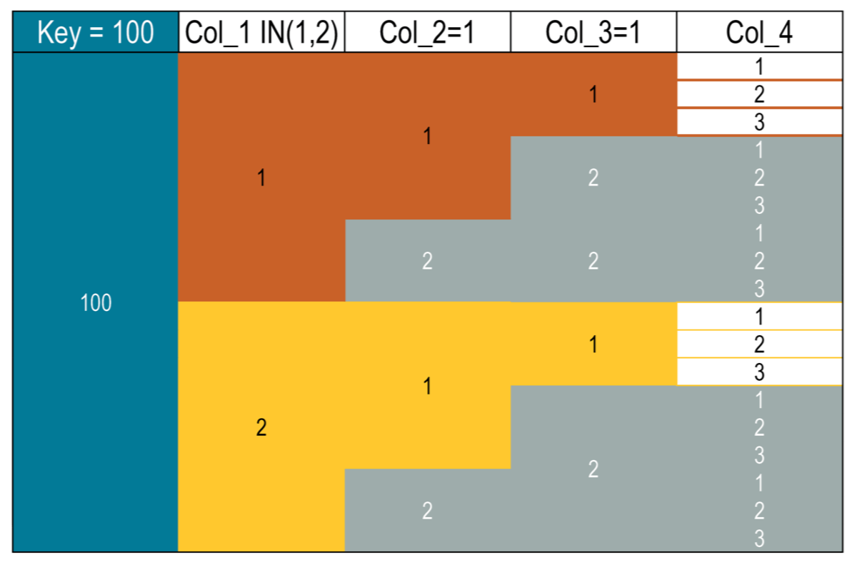
The results return the range from both segments:
 key | col_1 | col_2 | col_3 | col_4
-----+-------+-------+-------+-------
 100 |     1 |     2 |     2 |     1
 100 |     1 |     2 |     2 |     2
 100 |     1 |     2 |     2 |     3

(3 rows)
Clustering columns cannot be skipped but lower level columns can be omitted
Queries fail if they attempt to return ranges on the last clustering column without identifying any of the higher level clustering columns:
SELECT * FROM cycling.numbers WHERE key = 100 AND col_4 <= 2;The request is invalid:
InvalidRequest: Error from server: code=2200 [Invalid query] message=
"PRIMARY KEY column "col_4" cannot be restricted as preceding column "col_1" is not restricted"
However, unlike partition columns, a query can omit lower level clustering columns in logical statements as long as all preceding clustering columns are specified. For example, to filter one of the mid-level columns, restrict the first level column using equals or IN, then specify a range on the second level:
SELECT * FROM cycling.numbers WHERE key = 100 AND col_1 = 1 AND col_2 > 1Because the data hasn’t been filtered by all clustering columns, the database must scan through multiple segments to apply the specified conditions. This can be more resource-intensive that a fully specified query that restricts all clustering columns.
 key | col_1 | col_2 | col_3 | col_4
-----+-------+-------+-------+-------
 100 |     1 |     2 |     2 |     1
 100 |     1 |     2 |     2 |     2
 100 |     1 |     2 |     2 |     3

(3 rows)
Slice partitions with clustering columns
Uniquely, a WHERE clause can use clustering columns to retrieve a slice, which is a range of rows from a partition.
To retrieve a slice, the WHERE clause must include the clustering columns in the order that they are defined in the primary key.
The query locates a specific row using the ordered clustering columns, and then the query can quickly retrieve the rows before that row, after that row, or between two targeted rows (if two separate slice conditions are specified).
To retrieve a slice of a slice, narrow the range of rows with conditions on the higher level clustering columns (all except the last clustering column).
The syntax for a slice logical statement is as follows:
(clustering1, clustering2[, …]) <range_operator> (value1, value2[, …])
[AND (clustering1, clustering2[, …]) <range_operator> (value1, value2[, …])]
Slices must filter on all clustering columns to a single row at the lowest targeted level of the clustering hierarchy. The following statement identifies the row where column 1, 2, and 3 are equal to 2, and then it retrieves the slice of rows where column 4 is less than or equal to 1:
SELECT * FROM cycling.numbers
  WHERE key = 100 AND (col_1, col_2, col_3, col_4) <= (2, 2, 2, 1);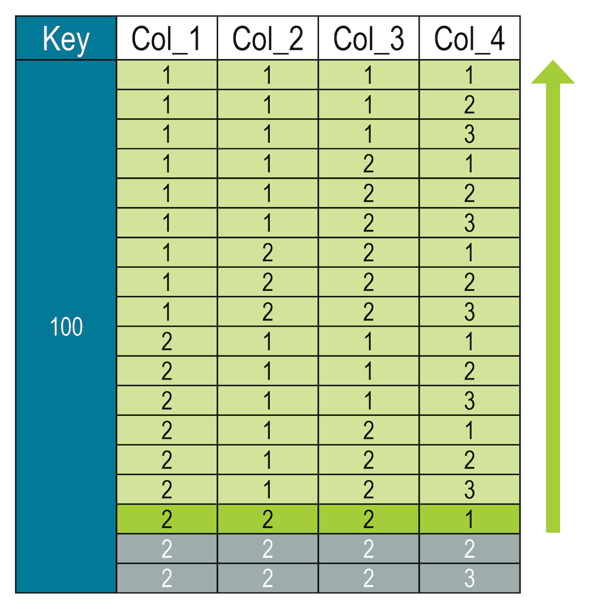
The database is NOT filtering on all values in column 4: It finds the exact location of one row (shown in dark green in the figure), and then it retrieves a range from that position. Earlier levels of the hierarchy (other columns) aren’t considered in the final range evaluation.
It is possible for the location to be hypothetical, meaning that the dataset doesn’t contain an exact match for the targeted row.
For example, the following query specifies slice values of (2, 1, 1, 4).
The value of column 4 is only evaluated to locate the row placement within the clustering segment.
The database locates the segment and then finds col_4 = 4.
After finding the location, it returns the row and all the rows before it in the sort order (which in this case spans all clustering columns).
SELECT * FROM cycling.numbers
  WHERE key = 100 AND (col_1, col_2, col_3, col_4) <= (2, 1, 1, 4);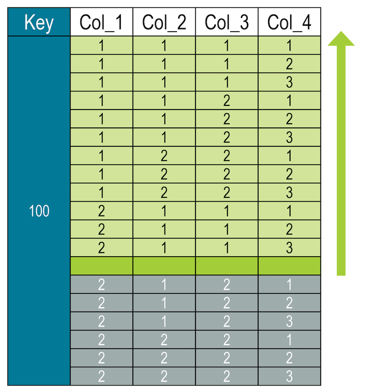
The same rules apply to slice restrictions when two slice conditions retrieve a slice between targeted rows: you must identify the higher level clustering segments exactly, and then specify a range on the lower segments.
For example, to return rows where the value is greater than (1, 3) and less than or equal to (2, 5):
SELECT * FROM cycling.numbers WHERE key = 100 AND col_1 = 1 AND col_2 = 1
  AND (col_3, col_4) >= (1, 2) AND (col_3, col_4) < (2, 3);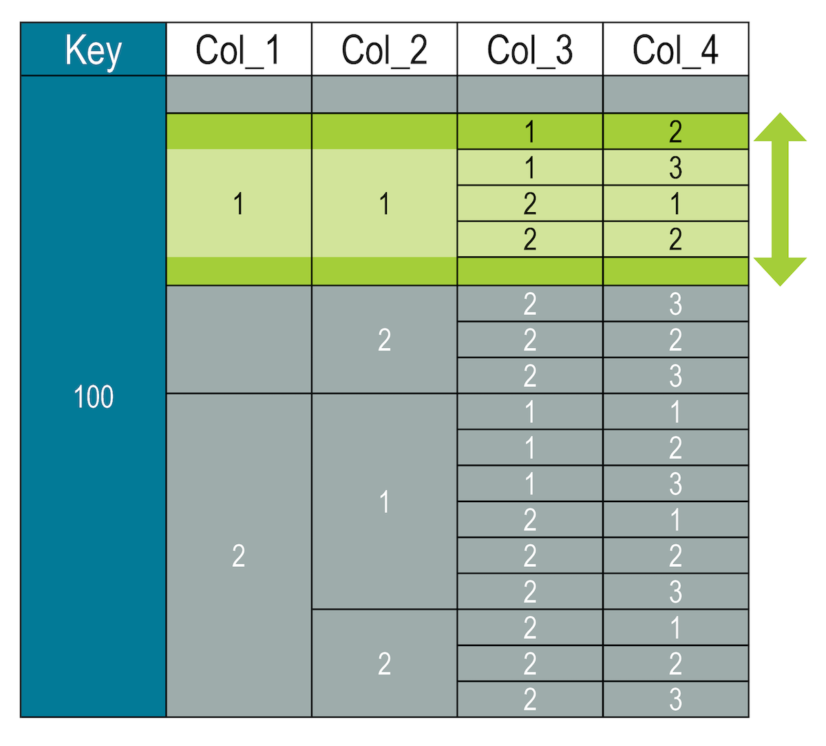
When returning a slice between two rows, the slice statements must define the same clustering columns. The query is rejected if the columns are different. For example, the following query is invalid because the slice ranges don’t define the same clustering columns.
SELECT * FROM cycling.numbers WHERE key = 100 AND col_1 = 1
  AND (col_2, col_3, col_4) >= (1, 1, 2)  AND (col_3, col_4) < (2, 3);
InvalidRequest: Error from server: code=2200 [Invalid query]
message="Column "col_3" cannot be restricted by two inequalities not starting
with the same column"|
You can force invalid queries with the |
You can slice multiple columns as long as each column has a complete slice range.
For example, the following table contains dates as integers, such as start_month = 1 for January.
This means that these columns can be sliced using a range.
CREATE TABLE IF NOT EXISTS cycling.events (
  year int,
  start_month int,
  start_day int,
  end_month int,
  end_day int,
  race text,
  discipline text,
  location text,
  uci_code text,
  PRIMARY KEY (
    (year, discipline), start_month, start_day, race
  )
);
The following query finds road cycling races that started between January 15th, 2017 and February 14th, 2017.
Notice that the query uses single values for the year and discipline columns, and slice ranges are defined on the start_month and start_day columns.
SELECT start_month as month, start_day as day, race FROM cycling.events
  WHERE year = 2017 AND discipline = 'Road'
    AND (start_month, start_day) < (2, 14)
    AND (start_month, start_day) > (1, 15);
The results contain events in the queried time period:
 month | day | race
-------+-----+-----------------------------------------------------------------
     1 |  23 |                      Vuelta Ciclista a la Provincia de San Juan
     1 |  26 | Cadel Evans Great Ocean Road Race - Towards Zero Race Melbourne
     1 |  26 | Challenge Mallorca: Trofeo Porreres-Felanitx-Ses Salines-Campos
     1 |  28 |                               Cadel Evans Great Ocean Road Race
     1 |  28 |          Challenge Mallorca: Trofeo Andratx-Mirador des Colomer
     1 |  28 |            Challenge Mallorca: Trofeo Serra de Tramuntana -2017
     1 |  29 |                               Cadel Evans Great Ocean Road Race
     1 |  29 |                                                      Dubai Tour
     1 |  29 |                             Grand Prix Cycliste la Marseillaise
     1 |  29 |                                Mallorca Challenge: Trofeo Palma
     1 |  31 |                                            Ladies Tour of Qatar
     2 |   1 |                                              Etoile de Besseges
     2 |   1 |                                           Jayco Herald Sun Tour
     2 |   1 |                                 Volta a la Comunitat Valenciana
     2 |   5 |                                       G.P. Costa degli Etruschi
     2 |   6 |                                                   Tour of Qatar
     2 |   9 |                                South African Road Championships
     2 |  11 |                                               Trofeo Laigueglia
     2 |  11 |                           Vuelta Ciclista a la Region de Murcia
     2 |  12 |                                              Clasica de Almeria

(20 rows)
GROUP BY clause
Group by one or more columns.
Condenses the selected rows that share the same values for a set of columns or values returned by a function into a group.
Either one or more primary key columns or a deterministic function or aggregate can be used in the GROUP BY clause.
SELECT race_date, race_time FROM cycling.race_times_summary
  GROUP BY race_date;
Each set of rows with the same race_date column value are grouped together into one row in the query output.
Three rows are returned because there are three groups of rows with the same race_date column value.
The value returned is the first value that is found for the group.
 race_date  | race_time
------------+--------------------
 2019-03-21 | 10:01:18.000000000
 2018-07-26 | 10:01:18.000000000
 2017-04-14 | 10:01:18.000000000

(3 rows)

Warnings :
Aggregation query used without partition key
This query groups the rows by race_date and FLOOR(race_time, 1h), which returns the hour.
The number of rows in each group is returned by COUNT(*).
SELECT race_date, FLOOR(race_time, 1h), COUNT(*) FROM cycling.race_times_summary
  GROUP BY race_date, FLOOR(race_time, 1h);
Nine rows are returned because there are nine groups of rows with the same race_date and FLOOR(race_time, 1h) values:
 race_date  | system.floor(race_time, 1h) | count
------------+-----------------------------+-------
 2019-03-21 |          10:00:00.000000000 |     2
 2019-03-21 |          11:00:00.000000000 |     1
 2019-03-21 |          12:00:00.000000000 |     1
 2018-07-26 |          10:00:00.000000000 |     2
 2018-07-26 |          11:00:00.000000000 |     1
 2018-07-26 |          12:00:00.000000000 |     1
 2017-04-14 |          10:00:00.000000000 |     2
 2017-04-14 |          11:00:00.000000000 |     1
 2017-04-14 |          12:00:00.000000000 |     1

(9 rows)

Warnings :
Aggregation query used without partition key
ORDER BY clause
You can fine-tune the display order using the ORDER BY clause.
The partition key must be defined in the WHERE clause and then the ORDER BY clause defines one or more clustering columns to use for ordering.
The order of the specified columns must match the order of the clustering columns in the PRIMARY KEY definition.
The options for ordering are ASC (ascending) and DESC (descending).
If no order is specified, the results are returned in the stored order.
To use ORDER BY with IN, you must disable paging with the CQL shell PAGING OFF command.
SELECT * FROM cycling.calendar WHERE race_id IN (100, 101, 102)
ORDER BY race_start_date ASC;
race_id | race_start_date | race_end_date | race_name
---------+---------------------------------+---------------------------------+-----------------------
100 | 2015-05-09 00:00:00.000000+0000 | 2015-05-31 00:00:00.000000+0000 | Giro d'Italia
100 | 2014-05-08 00:00:00.000000+0000 | 2014-05-30 00:00:00.000000+0000 | Giro d'Italia
100 | 2013-05-07 00:00:00.000000+0000 | 2014-05-29 00:00:00.000000+0000 | Giro d'Italia
102 | 2015-06-13 00:00:00.000000+0000 | 2015-06-21 00:00:00.000000+0000 | Tour de Suisse
102 | 2014-06-12 00:00:00.000000+0000 | 2014-06-20 00:00:00.000000+0000 | Tour de Suisse
102 | 2013-06-11 00:00:00.000000+0000 | 2013-06-19 00:00:00.000000+0000 | Tour de Suisse
101 | 2015-06-07 00:00:00.000000+0000 | 2015-06-14 00:00:00.000000+0000 | Criterium du Dauphine
101 | 2014-06-06 00:00:00.000000+0000 | 2014-06-13 00:00:00.000000+0000 | Criterium du Dauphine
101 | 2013-06-05 00:00:00.000000+0000 | 2013-06-12 00:00:00.000000+0000 | Criterium du Dauphine
103 | 2015-07-04 00:00:00.000000+0000 | 2015-07-26 00:00:00.000000+0000 | Tour de France
103 | 2014-07-03 00:00:00.000000+0000 | 2014-07-25 00:00:00.000000+0000 | Tour de France
103 | 2013-07-02 00:00:00.000000+0000 | 2013-07-24 00:00:00.000000+0000 | Tour de France
(12 rows)Vector search with ORDER BY
The ORDER BY clause also supports vector search on a vector column.
The result set is sorted using the approximate nearest neighbor (ANN) algorithm with the supplied array values.
This query uses a vector in the ORDER BY clause to run a similarity search on the table’s vector column:
SELECT * FROM cycling.comments_vs
  ORDER BY comment_vector ANN OF [0.15, 0.1, 0.1, 0.35, 0.55]
  LIMIT 3;
The response contains the rows that are most similar to the query vector, sorted by similarity:
 id                                   | created_at                      | comment                                | comment_vector               | commenter | record_id
--------------------------------------+---------------------------------+----------------------------------------+------------------------------+-----------+--------------------------------------
 e8ae5cf3-d358-4d99-b900-85902fda9bb0 | 2017-04-01 14:33:02.160000+0000 |              rain, rain,rain, go away! | [0.9, 0.54, 0.12, 0.1, 0.95] |      John | 6711e6c0-2f6a-11ef-bd2f-836fa334e187
 e7ae5cf3-d358-4d99-b900-85902fda9bb0 | 2017-04-01 14:33:02.160000+0000 | LATE RIDERS SHOULD NOT DELAY THE START | [0.9, 0.54, 0.12, 0.1, 0.95] |      Alex | 670c4170-2f6a-11ef-bd2f-836fa334e187
 e8ae5df3-d358-4d99-b900-85902fda9bb0 | 2017-04-01 14:33:02.160000+0000 |                    Rain like a monsoon | [0.9, 0.54, 0.12, 0.1, 0.95] |      Jane | 6712d120-2f6a-11ef-bd2f-836fa334e187

(3 rows)
LIMIT clause
If a query returns a large number of rows, you can limit the number of rows returned, to limit the amount of data returned.
The default limit is set to 10,000 rows, the number of rows cqlsh allows.
This examples limits the rows to 1:
SELECT created_at FROM cycling.comments
  WHERE id = e7ae5cf3-d358-4d99-b900-85902fda9bb0
LIMIT 1;
created_at
---------------------------------
2024-07-02 00:00:00.000000+0000
(1 rows)OFFSET option
The LIMIT clause can also use the OFFSET option to skip a number of rows before returning the results.
OFFSET cannot be used without LIMIT.
This is an expensive feature for large offsets and should be avoided.
Non-offset pagination is a better option for large datasets.
There are guardrail settings in the cassandra.yaml file that will prevent offsets that are too large.
The offset_rows_warn_threshold defaults to 10,000 rows. The offset_rows_failure_threshold defaults to 20,000 rows.
There are a number of restrictions on the use of OFFSET:
-
Specifying an OFFSET disables normal key-based paging.
-
Using
OFFSET 0also disables key-based paging. -
ANNqueries don’t supportOFFSET.
This example limits the rows to 3, but skips the first two rows:
SELECT comment,comment_vector,commenter FROM cycling.comments_vs
  WHERE commenter : 'Alex'
  LIMIT 3 OFFSET 2;
comment | comment_vector | commenter
----------------------------------------+-------------------------------+-----------
Raining too hard should have postponed | [0.45, 0.09, 0.01, 0.2, 0.11] | Alex
(1 rows)PER PARTITION LIMIT clause
The PER PARTITION LIMIT option sets the maximum number of rows that the query returns from each partition.
This will only apply to tables that spread across more than one partition.
An example of such a table is defined here:
USE cycling;
CREATE TABLE rank_by_year_and_name (
  race_year int,
  race_name text,
  cyclist_name text,
  rank int,
  PRIMARY KEY ((race_year, race_name), rank)
);
where the partition key is a composite of race_year and race_name.
The following query returns the top two cyclists from each partition stored:
SELECT rank, cyclist_name AS name FROM cycling.rank_by_year_and_name
  PER PARTITION LIMIT 2;
rank | name
------+----------------------
1 | Phillippe GILBERT
2 | Daniel MARTIN
1 | Daniel MARTIN
2 | Johan Esteban CHAVES
1 | Ilnur ZAKARIN
2 | Carlos BETANCUR
1 | Benjamin PRADES
2 | Adam PHELAN
(8 rows)ALLOW FILTERING
|
Unless you have an explicit, tested use case, don’t use |
The ALLOW FILTERING clause allows you to perform queries that require scanning all partitions, with no primary key columns specified.
These queries can be extremely long running and resource intensive, resulting in severe performance issues.
As a best practice, your data model should avoid queries that require ALLOW FILTERING.
For small datasets or testing purposes on small datasets, it can be useful, and it could help you identify where you need to add indexes to your data model.
The following query selects the birthday and nationality columns from the cyclist_alt_stats table, with the ALLOW FILTERING clause:
SELECT lastname, birthday, nationality FROM cycling.cyclist_alt_stats
  WHERE birthday = '1991-08-25' AND nationality = 'Ethiopia'
ALLOW FILTERING;
lastname | birthday | nationality
----------+------------+-------------
GRMAY | 1991-08-25 | Ethiopia
(1 rows)