Read request processing
To complete a read request, the DataStax Enterprise (DSE) database must combine results from the table’s memtable and one or more SSTables, depending on the compaction strategy and the distribution of data across SSTables. If the required partition data is found in multiple locations, the data is merged from the different sources to provide a complete view of the partition.
Finding the data for a read request is a multi-stage process known as the read path. This process starts by checking the memtable, and then checks several SSTable structures to locate the required data in memory or on disk:
-
Check the memtable.
-
Check the row cache, if enabled.
-
Check the bloom filter.
-
Check the partition key cache, if enabled.
-
If a partition key is found in the partition key cache, get the compression offset map.
If a partition key isn’t in the partition key cache:
+ .. Check the partition summary for the partition key range. .. Use the range to check the partition index for the partition key location. .. Get the compression offset map.
-
Use the compression offset map to locate the data on disk.
-
Fetch the data from the SSTable on disk.
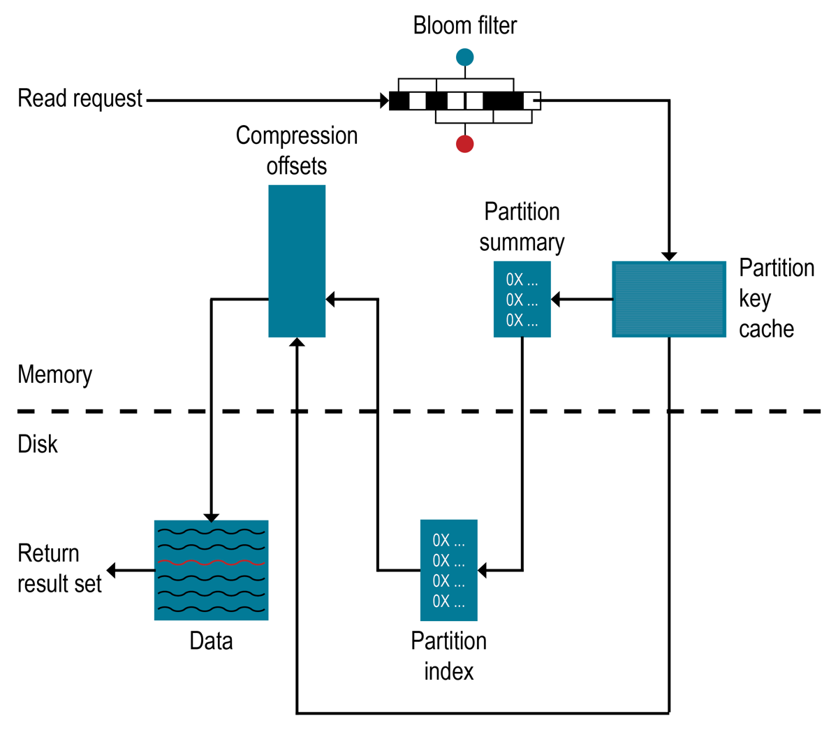
|
The read path doesn’t access every structure for every read. Various caches allow the database to bypass certain steps by pulling from cache instead of finding and reading data on disk. |
Row cache
All databases read fastest when the most frequently accessed data fits into memory.
Generally, the OS page cache is best at improving performance. In some cases, the row cache can improve workloads where the overwhelming majority of requests are reads (approximately 95 percent). Row cache isn’t recommended for write-heavy workloads.
If you enable the row cache, it stores a subset of the partition data on disk in SSTables in memory. If this data is needed for a read, it is read from the row cache, eliminating the need to retrieve that data from disk. If a row must be retrieved from disk (SSTables), the compiled row is added to the row cache in case it is needed again.
The row cache is stored in fully off-heap memory using an implementation that relieves garbage collection pressure in the Java Virtual Machine (JVM). Data stored in the row cache uses a configurable amount of memory for a specified period of time. When the cache is full, the row cache uses least-recently-use (LRU) eviction to reclaim memory. This inherently results in the row cache populating with the most frequently read rows.
You can configure the row cache size and the number of rows to store. Storing a set number of rows is a useful feature that can make queries like "Last 10 items" very fast to read.
The row cache is not write-through. If a write mutates a cached row, the cached row is invalidated, and it isn’t cached again until the row is read again. Similarly, if a partition is updated, the entire partition is removed from the cache. If required partition data isn’t found in the row cache, then the database checks bloom filters.
Bloom filter
Each SSTable has an associated bloom filter that can establish whether certain partition data is present in that SSTable. Bloom filters improve the performance of partition key lookups during reads by narrowing the pool of keys for a given SSTable. Bloom filters are used for index scans, not range scans.
The database checks the bloom filter to discover which SSTables are likely to have the requested partition data. If the bloom filter doesn’t explicitly exclude a particular SSTable, then the database checks the partition key cache.
Not all SSTables identified by a bloom filter will have the predicted data. Because the bloom filter is a probabilistic function, it can sometimes return false positives.
The bloom filter is stored in off-heap memory, and it can use as much as 1 to 2 GB per billion partitions. In an extreme case, each row can have a partition, so one machine could have billions of these entries.
Tuning bloom filter settings can help balance memory usage and performance (successful lookups). For more information, see Tune bloom filters.
Partition Key Cache
If the partition key cache is enabled, it stores a partition index cache in off-heap memory. If a cached partition key is needed for a read, it is pulled from the partition index cache, eliminating the need to search the partition summary and then read from the partition index. Using the cached partition key, the DSE database refers directly to the compression offset map to find the compressed block on disk that has the data.
The partition key cache performs best when warm (not empty), and a warm partition key cache can significantly improve read performance compared with cold-start (empty cache) reads. To warm the partition key cache, you can run some preset reads at startup to access known hot partition keys, ensuring they are loaded into the cache before receiving a live request.
The partition key cache uses a small, configurable amount of memory; however, if memory is very limited on a node, you can limit the number of partition keys saved in the key cache. For more information, see Configure data caches.
Partition Summary
The partition summary is an off-heap, in-memory structure that stores samples of the partition index known as partition key ranges. The partition summary doesn’t provide the exact location of a partition key, but the partition summary can help the database find the required partition key range faster.
Whereas the partition index contains all partition keys, the partition summary samples segments of keys and maps their location in the index file. For example, if the partition summary is set to sample every 20 keys, it stores the location of the first key as the beginning of the SSTable file, the 20th key and its location in the file, and so on. This sampling helps the database find the range of partition keys that might contain the required key, reducing the search space in the partition index. After finding the range of possible partition key values, the database searches that range in the partition index.
You can configure the sample frequency to balance memory usage and read performance.
The granular sampling requires more memory to cache more ranges.
To configure the sampling frequency, set the min_index_interval and max_index_interval table properties when you create or alter a table.
To configure the amount of memory allocated to the partition summary, use the index_summary_capacity_in_mb parameter in cassandra.yaml.
Partition index
The partition index is stored on disk, and it contains an index of partition keys mapped to their offset.
After the database checks the partition summary for a range of partition keys, it searches for the required partition key in the partition index. The database runs one seek and sequential read of the columns over the given range. The information in the partition index is used to retrieve the compression offset map, and then find the compressed block on disk that has the actual row data.
Compression offset map
The compression offset map stores pointers to the exact location on disk where the desired partition data is stored. This location is stored in off-heap memory, and it is accessed by either the partition key cache or the partition index.
Once the database knows the location on disk, it fetches the compressed partition data from the relevant SSTables. Then, the database prepares the result set for the original read request. Depending on caching configuration, the database also uncompresses retrieved data and stores it in memory.
|
Within a partition, all rows aren’t equally expensive to query. The beginning of the partition (the first rows, clustered by the table’s key definition) is slightly less expensive to query because there is no need to consult the partition index. |
The compression offset map can increase as much as 1 to 3 GB for each TB of compressed data. More compressed data requires more compressed blocks, resulting in a larger compression offset table to map the blocks.
In DSE, compression is enabled by default even though finding blocks in the compression offset map consumes CPU resources. The OS page cache is more effective with compression enabled, typically resulting in faster reads.
Write patterns affect read performance
Write operations can affect the performance of read operations in a cluster. For example, compaction strategies that are best for read-heavy workloads minimize the number of SSTables and make reads more efficient because there are fewer files to check on the read path. In contrast, strategies that are best for write-heavy workloads create more SSTables, which can make reads take longer to complete.
