How is data maintained?

The DataStax Enterprise (DSE) database write process stores data in files called SSTables. SSTables are immutable. Instead of overwriting existing rows with inserts or updates, the database writes new timestamped versions of the inserted or updated data in new SSTables. The database does not perform deletes by removing the deleted data. Instead, the database marks deleted data with tombstones.

Over time, the database may write many versions of a row in different SSTables. Each version may have a unique set of columns stored with different timestamps. As SSTables accumulate, the distribution of data can require accessing more and more SSTables to retrieve a complete row.

To keep the database healthy, the database periodically merges SSTables and discards old data. This process is called compaction.

Compaction

Compaction works on a subset of SSTables. From these SSTables, compaction collects all versions of each unique row and assembles one complete row, using the most up-to-date version (by timestamp) of each of the row’s columns. The merge process is performant, because rows are sorted by partition key within each SSTable, and the merge process does not use random I/O. The new version of each row is written to a new SSTable. The old versions, along with any rows that are ready for deletion, are left in the old SSTables, and are deleted when any pending reads are completed.

How compaction works

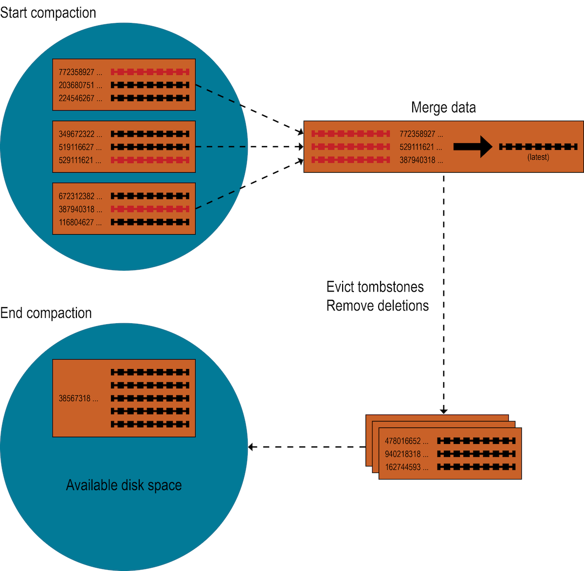
Compaction causes a temporary spike in disk space usage and disk I/O while old and new SSTables co-exist. As it completes, compaction frees up disk space occupied by old SSTables. It improves read performance by incrementally replacing old SSTables with compacted SSTables. The database can read data directly from the new SSTable even before it finishes writing, instead of waiting for the entire compaction process to finish.

DSE provides predictable high performance even under heavy load by replacing old SSTables with new ones in memory as it processes writes and reads. Caching the new SSTable, while directing reads away from the old one, is incremental and does not cause a the dramatic cache miss storm.

Compaction strategies

The DSE database supports different compaction strategies. These strategies control which SSTables are chosen for compaction and how the compacted rows are sorted into new SSTables. Each strategy has its own strengths. The sections that follow explain each compaction strategy.

Although each of the following sections starts with a generalized recommendation, many factors complicate the choice of a compaction strategy. See Choosing a compaction strategy.

UnifiedCompactionStrategy (UCS)

Recommended for use in DSE 6.8.25+ clusters with any workload, but especially with vertically scaled nodes. UCS behaves similarly, but better than STCS or LCS compaction strategies, due to implementation differences.

Pros: Useful for any workload. Unifies and improves tiered (STCS) and leveled (LCS) compaction strategies. Utilizes sharding (partitioned data compacted in parallel). Provides configurable read, write amplification guarantees. Parameters are reconfigurable at any time. UCS reduces disk space overhead and is stateless.

Consider using UCS if your legacy compaction strategy is not optimum.
Cons: UCS behavior is not meant to mirror TWCS’s append-only time series data compaction.

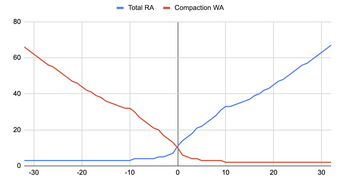
Use UnifiedCompactionStrategy (UCS) to adjust the balance between the number of SSTables that need to be consulted to serve a read (in other words, the database’s read amplification, RA) versus the number of times a piece of data must be rewritten during its lifetime (in other words, the database’s write amplification, WA). Configure UCS with a single scaling parameter which determines the compaction mode (positive values select tiered mode and negative values select leveled mode) and the compaction hierarchy’s fan factor F. The strategy organizes data in a hierarchy of levels defined by the size of SSTables. Each level accepts SSTables that are between a given size and F times that size. In leveled mode, compaction is triggered immediately when more than one SSTable is present on a level. In tiered mode, compaction is triggered as the threshold of F times a given size is reached or exceeded. The results vary per mode. At each level in leveled mode, UCS recompacts data multiple times with the goal to maintain one SSTable per level. In tiered mode UCS compacts only once but maintains multiple SSTables.

Change the behavior of UCS to be more like STCS or LCS with one scaling factor (W) parameter. This may be set per level. Because levels can be set to different values of W, levels can behave differently. For example, level zero (0) could behave like STCS but higher levels could increasingly behave like LCS.

UCS scaling factor W

The W scaling factor is an integer parameter that determines read (RA) and write (WA) amplification bounds and STCS versus LCS behavior. The W factor is set accordingly:

W < 0 = LCS where W = -8 emulates an improved LCS mode (leveled compactions with high WA, but low RA).
W = 0 - middle ground (leveled and tiered compactions behave identically).
W > 0 ⇒ STCS where W = 2 emulates an improved STCS mode (tiered compactions with low WA, but high RA)

The default is W = 2 for all levels. UCS tries not to recompact on a scaling factor change. Set incremental changes to minimize the impact.

The parameters of UCS can be changed at any time. For example, an operator may decide to:

decrease the scaling parameter, lowering the read amplification at the expense of more complex writes when a certain table is read-heavy and could benefit from reduced latencies.
increase the scaling parameter, reducing the write amplification, when it has been identified that compaction cannot keep up with the number of writes to a table.

Any such change only initiates compactions that are necessary to bring the hierarchy in a state compatible with the new configuration. Any additional work already done (for example, when switching from negative parameter to positive), is advantageous and incorporated.

In addition, UCS splits data on specific token boundaries when the data exceeds a set size and forms independent compaction hierarchies in each shard. This reduces the size of the largest SSTables in the node. For example, instead of one 1-TB SSTable there are 10 shards, each with 100-GB. Sharding also permits UCS to execute compactions in each shard independently and in parallel, which is crucial to keep up with the demands of high-density nodes. UCS can apply whole-table expiration, which proves useful for time-series data with time-to-live constraints.

UCS selection of SSTable levels is more stable and predictable than that of SizeTieredCompactionStrategy (STCS). STCS groups SSTables by size, whereas UCS groups by timestamp. UCS efficiently tracks time order and whole table expiration.

UCS and LCS compaction strategies end with similar results. However, UCS handles the problem of space amplification by sharding on specific token boundaries. LCS splits SSTables based on a fixed size with boundaries usually falling inside SSTables on the next level, kicking off compaction more frequently than necessary. Therefore UCS aids with tight write amplification control.

Parameters control the choice of different ratios of read and write amplification. Choose options that favor leveled compaction to improve reads at the expense of writes, or tiered compaction that favor writes at the expense of reads. Contact your DataStax account team for details.

SizeTieredCompactionStrategy (STCS)

Recommended for write-intensive workloads.

Pros: Compacts write-intensive workload very well.
Cons: Can hold on to stale data too long. Required memory increases over time.

The SizeTieredCompactionStrategy (STCS) initiates compaction when the database has accumulated a set number (default: 4) of similar-sized SSTables. STCS merges these SSTables into one larger SSTable. As the larger SSTables accumulate, STCS merges these into even larger SSTables. At any given time, several SSTables of varying sizes are present.

Maintain STCS

While STCS works well to compact a write-intensive workload, it makes reads slower because the merge-by-size process does not group data by rows. This makes it more likely that versions of a particular row may be spread over many SSTables. Also, STCS does not evict deleted data predictably because its trigger for compaction is SSTable size, and SSTables might not grow quickly enough to merge and evict old data. As the largest SSTables grow in size, the amount of disk space needed for both the new and old SSTables simultaneously during STCS compaction can outstrip a typical amount of disk space on a node.

LeveledCompactionStrategy (LCS)

Recommended for read-intensive workloads.

Pros: Disk requirements are easier to predict. Read operation latency is more predictable. Stale data is evicted more frequently.
Cons: Much higher I/O utilization impacting operation latency

The LeveledCompactionStrategy (LCS) alleviates some of the read operation issues with STCS. This strategy works with a series of levels. First, data in memtables is flushed to SSTables in the first level (L0). LCS compaction merges these first SSTables with larger SSTables in level L1.

Leveled compaction part 1

The SSTables in levels greater than L1 are merged into SSTables with a size greater than or equal to sstable_size_in_mb (default: 160 MB). If a L1 SSTable stores data of a partition that is larger than L2, LCS moves the SSTable past L2 to the next level up.

Leveled compaction part 2

In each of the levels above L0, LCS creates SSTables that are about the same size. Each level is 10 times the size of the last level, so level L1 has 10 times as many SSTables as L0, and level L2 has 100 times as many as L0. If the result of the compaction is more than 10 SSTables in level L1, the excess SSTables are moved to level L2.

Keep in mind that the maximum overhead when using LCS is the sum of N-1 levels. For example, given a maximum table size of 160 megabytes, once past level 3, overhead requirements expand drastically from 1.7 terabytes at level 4 to 17 terabytes at level 5:

L0 1      * 160 MB = 160 MB
L1 10     * 160 MB = 1600 MB
L2 100    * 160 MB = 16000 + 1600 = 17 GB
L3 1000   * 160 MB = 160000 + 1600 + 16000 =  177 GB
L4 10000  * 160 MB = 1600000 + 1600 + 16000 + 160000 =  1.7 TB
L5 100000 * 160 MB = 16000000 + 1600 + 16000 + 160000 + 1600000 =  17 TB

To mitigate that situation, switch to STCS and add additional nodes or reduce the sstable size using sstablesplit.

The LCS compaction process guarantees that the SSTables within each level starting with L1 have non-overlapping data. For many reads, this process enables the database to retrieve all the required data from only one or two SSTables. In fact, 90% of all reads can be satisfied from one SSTable. Since LCS does not compact L0 tables, however, resource-intensive reads involving many L0 SSTables may still occur.

At levels beyond L0, LCS requires less disk space for compacting: generally, 10 times the fixed size of the SSTable. Obsolete data is evicted more often, so deleted data uses smaller portions of the SSTables on disk. However, LCS compaction operations take place more often and place more I/O burden on the node. For write-intensive workloads, the payoff of using this strategy is generally not worth the performance loss to I/O operations. In many cases, tests of LCS-configured tables reveal I/O saturation on writes and compactions.

For additional information, see this presentation from Cassandra Summit 2016 and the associated YouTube video.

The database bypasses compaction operations when bootstrapping a new node using LCS into a cluster. The original data is moved directly to the correct level because there is no existing data, so no partition overlap per level is present. For more information, see the Apache Cassandra 2.2 - Bootstrapping Performance Improvements for Leveled Compaction blog.

TimeWindowCompactionStrategy (TWCS)

Recommended for time series and expiring time-to-live (TTL) workloads.

Pros: Well-suited for time series data, stored in tables that use the default TTL for all data. Simpler configuration than that of DateTieredCompactionStrategy (DTCS), which is deprecated in favor of TWCS.
Cons: Not appropriate if out-of-sequence time data is required, because SSTables will not compact well. Also, not appropriate for data without a TTL workload, as storage will grow without bound. Less fine-tuned configuration is possible than with DTCS.

The TimeWindowCompactionStrategy (TWCS) is similar to DTCS with simpler settings. TWCS groups SSTables using a series of time windows. During compaction, TWCS applies STCS to uncompacted SSTables in the most recent time window. At the end of a time window, TWCS compacts all SSTables that fall into that time window into a single SSTable based on the SSTable maximum timestamp. After the major compaction for a time window is completed, no further compaction of the data occurs, although tombstone compaction can still be run on sstables after the compaction_window threshold has passed. The process starts over with the SSTables written in the next time window.

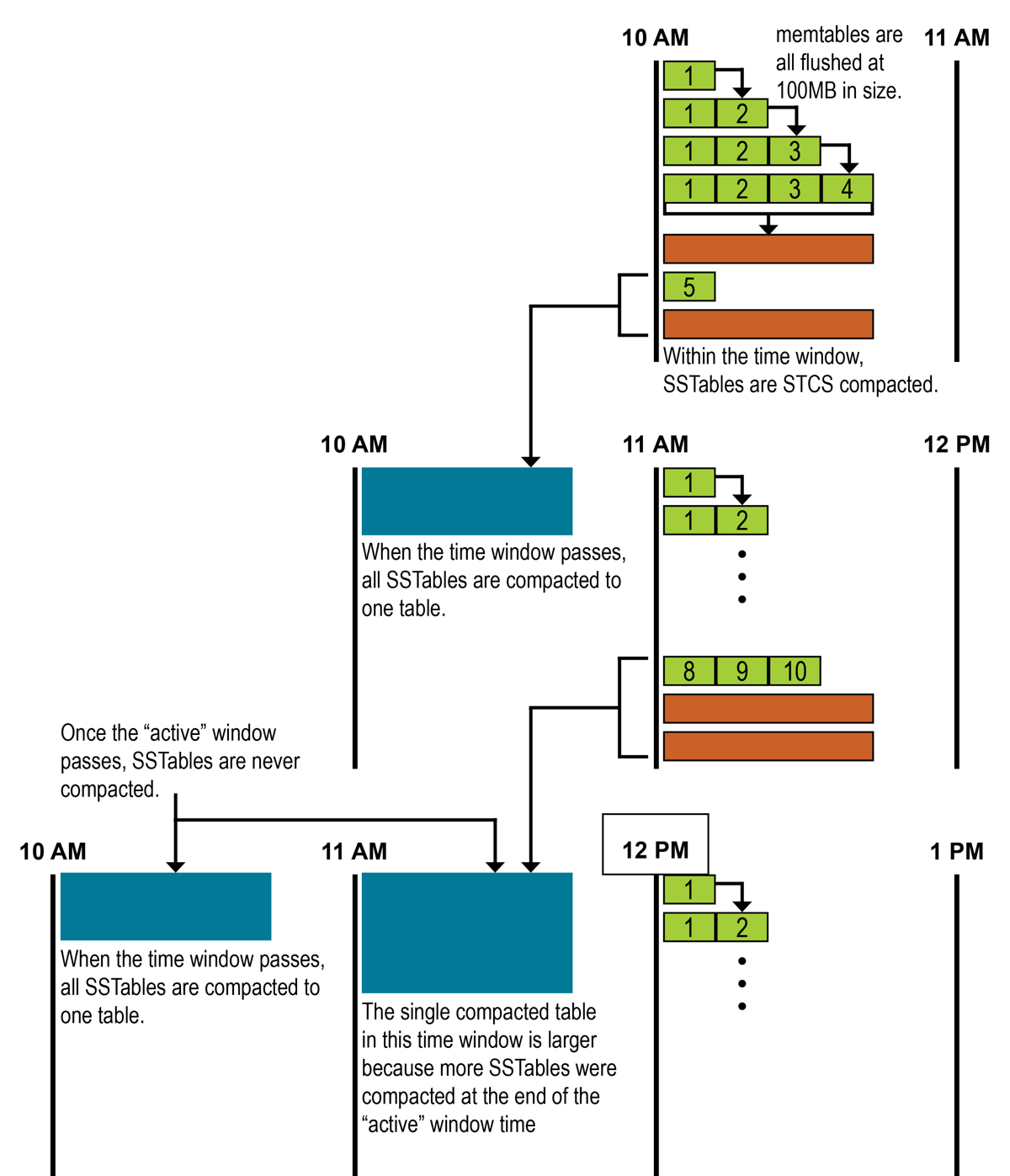
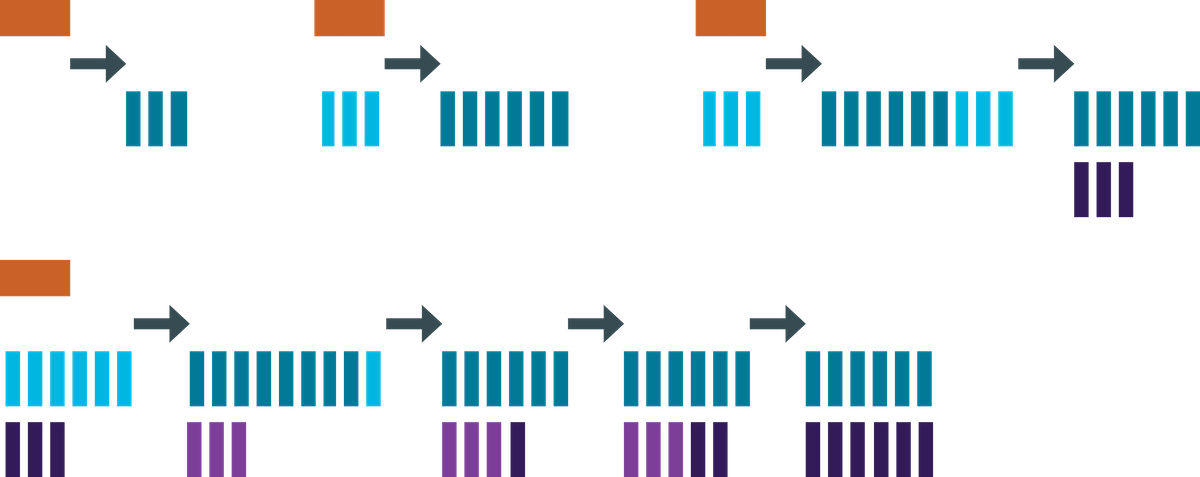
For tables where all cells have a time-to-live (TTL) applied, or tables using the default TTL, once all TTLs are passed, the gc_grace_seconds period has expired, and the droppable tombstone ratio is 100%, the sstable can be dropped without a compaction.

How TimeWindowCompactionStrategy works

As the figure shows, from 10 AM to 11 AM, the memtables are flushed from memory into 100MB SSTables. These SSTables are compacted into larger SSTables using STCS. At 11 AM, all these SSTables are compacted into a single SSTable, and never compacted again by TWCS.

At 12 PM, the new SSTables created between 11 AM and 12 PM are compacted using STCS, and at the end of the time window, the TWCS compaction repeats. Notice that each TWCS time window contains varying amounts of data.

For an animated explanation, see the DataStax Time Window Compaction Strategy video.

The TWCS configuration has two main property settings:

compaction_window_unit: time unit used to define the window size (milliseconds, seconds, hours, and so on)
compaction_window_size: how many units per window (1, 2, 3, and so on)

The configuration for the above example: compaction_window_unit = ‘minutes’,compaction_window_size = 60

DateTieredCompactionStrategy (DTCS) - Deprecated

Use TimeWindowCompactionStrategy (TWCS) instead.

The DateTieredCompactionStrategy (DTCS) is similar to STCS. But instead of compacting based on SSTable size, DTCS compacts based on SSTable age. Each column in an SSTable is marked with the timestamp at write time. As the age of an SSTable, DTCS uses the oldest (minimum) timestamp of any column the SSTable contains.

More information about compaction

The following blog posts and videos provide more information from developers who have tested compaction strategies: