Data model
Data modeling in Cassandra-based databases, like DataStax Enterprise (DSE), is different from relational databases. By design, Cassandra tables aren’t stored entirely on a single node or in complete copies on multiple replica nodes. Instead, data is divided into partitions that are allocated to replica nodes for storage. Because data is distributed across nodes, it’s important to understand this architecture, and then plan your data model and queries with respect to this architecture for optimal performance and scalability.
Keyspaces
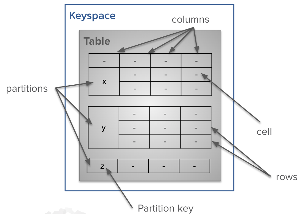
A keyspace is the outermost grouping of data within a database. Each table belongs to only one keyspace, and each keyspace can contain one or more tables. Keyspaces can also store other high-level database objects, such as custom types (user-defined types).
Typically, a cluster has one keyspace per application with many tables inside that keyspace, but keyspaces are not a significant map layer within the data model. However, the replication strategy is set at the keyspace level, and then applied to all tables within that keyspace. Data with different replication requirements must be stored in separate keyspaces.
Tables, columns, and rows
Tables are defined as rows of related data organized into columns. Each column has a data type set in the table definition. Rows consist of cells that contain the values stored in each column. A value in a cell must conform to the data type defined for the column. The unique identifier for a row is determined by the columns in the table’s primary key.
The table definition also includes properties for compaction, compression, and other mechanisms. For examples and more information, see CREATE TABLE.
When used to store schemaless data with the Data API, the table is called a collection, the columns are called fields, and the rows are called documents.
Table-per-query and denormalization
Typically, tables are designed to facilitate specific query patterns required by an application.
The table-per-query pattern is a common best practice in Cassandra-based databases. When designing a table, you choose the partition key, clustering columns, and any indexes to optimize for a specific query. Because Cassandra-based databases do not support joins, all the data required for a query must reside in a single table.
Attempting to create a single table that supports all queries introduces unnecessary complexity and inefficiency. Similarly, indexes aren’t a substitute for designing tables around queries; excessive use of indexes degrades performance.
When considering a new query, create a new table for it rather than adapting an existing one. This approach allows you to optimize each table for a specific query, improving both performance and scalability. It also helps keep the data model simple and maintainable, as each table has a clear purpose and structure.
The table-per-query pattern in Cassandra-based databases naturally leads to denormalization, which is the practice of duplicating data across multiple tables to optimize query performance. Since all data for a query must be contained within a single table, you may need to duplicate data across multiple tables to support different queries. In some cases, you will design multiple tables with exactly the same data, but with different partition keys and clustering columns to optimize different queries.
For example, consider an application that needs to query employee data by department and also by location.
The table-per-query pattern would lead to two separate tables, one for each query.
In this case the tables would contain the same data, but different partition keys and clustering columns.
A common naming convention for these tables is to use the query name as the table name, such as employees_by_department and employees_by_location.
The employees_by_department table uses the user-defined type CONTACT_INFO to store contact information for each employee.
This table supports the following query:
SELECT * FROM employees_by_department WHERE department = 'Engineering';
CREATE TABLE employees_by_department (
    department TEXT,
    last_name TEXT,
    first_name TEXT,
    employee_id int,
    start_date DATE,
    location TEXT,
    contact_info CONTACT_INFO,
    PRIMARY KEY ((department), last_name, first_name, employee_id)
);
The employees_by_location table uses the same data, but with a different partition key and clustering columns.
This table supports the following query:
SELECT * FROM employees_by_location WHERE location = 'New York';
CREATE TABLE employees_by_location (
    location TEXT,
    last_name TEXT,
    first_name TEXT,
    employee_id int,
    start_date DATE,
    department TEXT,
    contact_info CONTACT_INFO,
    PRIMARY KEY ((location), last_name, first_name, employee_id)
);
Primary keys
In Cassandra-based databases, a primary key uniquely identifies a row. The primary key is set in the table definition, and it consists of the partition key and optional clustering columns. Most tables should use a composite primary key (a partition key and clustering columns) to allow multiple rows to be stored within a single partition.
|
The primary key is immutable after creating a table. To change the primary key, you must create a new table schema, and then rewrite the existing data to the new table. |
Primary keys are critical to reading, writing, and distributing data efficiently. When defining the table’s primary key, consider the following:
-
The size of the partitions and the distribution of the partitions across nodes in the cluster
-
The primary key cannot have a
NULLvalue in any row -
The cardinality of the values in the primary key columns
-
The order of the data within partitions (set by the clustering columns)
The following sections provide more information about these considerations.
Partition keys
A partition key consists of the first column or set of columns in a primary key. All rows with the same partition key are stored in the same partition. Rows in the same partition are organized for efficient retrieval. To retrieve data from a table, the query must specify values for all columns defined in the partition key unless an index is created.
The database uses the partition key as input to a hashing function to determine which node in the cluster stores the partition. Queries use the partition key and the same hashing function to locate the partition and retrieve the data. This prevents the database from scanning all nodes in the cluster to find data.
If the partition key has only one column, it is known as a simple partition key. If there are no clustering columns (meaning, the entire primary key has only one column), all partitions have exactly one row.
Composite partition keys (bucketing)
In contrast to a simple partition key, a composite partition key uses two or more columns to identify where data resides. A composite partition key splits a dataset into chunks, also known as buckets, so that related data is stored on separate partitions. To facilitate retrieval, composite partition key columns delineate logical sets inside a partition.
Bucketing can help prevent unbounded growth in partitions and address write amplification on clusters that experience hotspotting or congestion by writing data to one node repeatedly. Bucketing involves adding a column to the partition key to split large partitions into smaller, more manageable ones. For proper load balancing, it is critical that your partition keys identify rows in such a way that evenly distributes the data while also enabling required query patterns.
The following example shows IoT data from a sensor without bucketing.
If one sensor sends data at a higher frequency than others, the partition for that sensor can grow very large.
The partition key is the sensor_id, and the rows are ordered by timestamp.
Each time a new temperature is received, the partition for the high-frequency sensor grows larger.
CREATE TABLE sensor_data (
    sensor_id UUID,
    timestamp TIMESTAMP,
    temperature FLOAT,
    PRIMARY KEY ((sensor_id), timestamp)
);
This is the same table, but with bucketing applied.
The partition key now contains a day column, so each partition contains data for a single day only.
CREATE TABLE sensor_data (
    sensor_id UUID,
    day DATE,
    timestamp TIMESTAMP,
    temperature FLOAT,
    PRIMARY KEY ((sensor_id, day), timestamp)
);
Cardinality
The columns chosen for a composite partition key must have sufficient cardinality to distribute data evenly across partitions.
Some data types inherently have low cardinality, such as boolean and tinyint.
This can lead to uneven distribution of data between partitions (nodes).
For example, the boolean type has only 2 possible values, so the table has only 2 partitions.
While large partitions are possible with any data type, low cardinality types are more prone to large partitions.
|
Be cautious when using the |
Clustering columns
Clustering columns are optional columns in the primary key.
Clustering columns sort the data so that multiple rows within a single partition are clustered in a defined order.
The clustering columns do not dictate the storage location of the data, only the order of the data within a partition.
Sorting within a partition can be useful, for example, if your queries need to retrieve sorted data, such as recent transactions, time series data, or events grouped by status (like pending and completed).
When creating a table, the partition key must precede the clustering columns. The first column declared in the key definition cannot also be a clustering column. If a table has no clustering columns, the partition key is the primary key.
A primary key with at least one clustering column is considered a compound primary key, and the resulting table is comprised of multi-row partitions. The table can be queried to return sorted results based on the clustering columns. For retrieval, queries should use the same sort order as the clustering columns. Reversing the sort order is inefficient because it can require full partition scans and re-sorting in memory.
Grouping data in tables using a clustering column or columns is analogous to JOINs in a relational database, but clustering columns are much more performant because only one table is accessed.
On a physical node, retrieval is more efficient because, for a given partition key, rows are stored in order based on the clustering columns.
Data modeling methodology
The data modeling methodology for Cassandra-based databases is a five-part process:
-
Create a conceptual data model.
-
Create an application workflow.
-
Use your conceptual data model and application workflow to create a logical data model.
-
Add implementation details to the logical data model to create a physical data model.
-
As application development continues, regularly optimize and tune your data model.
The following sections explain each part of the data modeling process. A simple video-sharing application is used as an example.
Create the conceptual data model
A conceptual data model is a high-level representation of the data and the relationships between different entities. This model should be business-centric and technology-agnostic:
-
Focus on how your business views the data, not how the data is stored or queried.
-
Reflect real-world business concepts and how they relate to each other, such as customers and products.
-
Avoid specific implementation details like data types or database systems.
Conceptual data models are often illustrated using an entity-relationship (ER) diagram that visually represents entities, such as users or product categories, and the relationships between them.
The following ER diagram represents a simple conceptual data model for a video-sharing application:
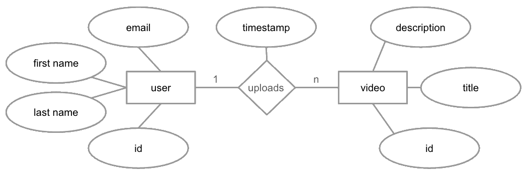
From a business operations perspective, the application expects that users will upload videos. In the diagram, the user entity is connected to the video entity by an upload action. Then, relevant data are attached to each of these three central nodes. For example:
-
The user entity has user-specific data like email, name, and ID.
-
The upload action has timestamp data.
-
The video entity has video-specific data like title, ID, and description.
This is a simple example. A conceptual data model for a real-world application would include many more entities, relationships, and data.
Create the application workflow
The application workflow identifies the essential queries that the application must support to deliver its functionality. These queries help define how users will interact with the system, and they guide the structure of your logical and physical data models.
You can write your application workflow queries in plain sentences, similar to user stories. For a video-sharing application, typical queries might include the following:
-
Find all videos uploaded by a user.
-
Upload a video.
-
Modify a video description.
-
Find all uploads for a user within a specific time range, sorted by most recent upload first.
Create the logical data model
The logical data model combines the entities and relationships from the conceptual data model with the queries defined in the application workflow. It defines tables, key columns, user-defined types, and indexes. For example:
| Query | Table name | Columns | Partition key | Clustering column |
|---|---|---|---|---|
Find all uploads for a user within a specific time range, sorted by most recent upload first |
|
|
|
|
Because the query retrieves uploads by a single user, the user_id column is set as the partition key.
Then, because the results are ordered by upload time, the upload column is set as a clustering column sorted in descending order.
The model also includes other video and user metadata columns in the table, even thought they don’t directly address the query.
This data is valuable to the response passed to the user so the user can understand the results.
Create the physical data model
The physical data model adds implementation-specific details to the logical model, including the data types needed to define tables and columns. You can translate the physical data model directly into CQL statements to create tables and indexes.
|
It is important that you choose appropriate data types for the actual values stored in each column. Misusing data types can lead to inefficient storage, poor performance, and inaccurate or failed queries. For information about the available data types and their usage, see CQL data types. |
The following example builds on the videos_by_user table from the previous logical model by specifying data types for each column:
| Column | Data type | Explanation |
|---|---|---|
|
|
Ensures each user is uniquely identified. |
|
|
Ensures the upload time is recorded.
|
|
|
Ensures each video has a globally unique identifier. |
|
|
Stores the user’s email address. Uniqueness not enforced since a user can upload multiple videos. |
|
|
Stores the user’s first name. Uniqueness not enforced. |
|
|
Stores the user’s last name. Uniqueness not enforced. |
|
|
Stores the video’s title. Uniqueness not enforced. |
|
|
Stores the video’s description. Uniqueness not enforced. |
After creating the physical data model, you have a mapping for the resulting CQL CREATE TABLE statement.
For example:
CREATE TABLE videos_by_user (
  user_id uuid,
  upload timestamp,
  video_id uuid,
  email text,
  first_name text,
  last_name text,
  title text,
  description text,
  PRIMARY KEY ((user_id), upload)
);
Data model tuning and optimization
Data modeling is iterative. As your application evolves, you might need to revisit and refine the data model to maintain performance, scalability, and functionality. Common reasons for revisiting the model include shifting business priorities, introduction of new features in the application, and performance issues.
Monitor database performance to identify potential bottlenecks and areas for optimization. If queries begin to slow down or resource usage increases, adjustments to partitioning, indexing, or data layout may be necessary to restore optimal performance. For example:
- Imbalanced partitions
-
As a dataset grows over time or your query patterns change without corresponding changes to the data model, partitions can become imbalanced. This creates hot spots where some nodes carry a heavier load than others. Techniques like bucketing can rebalance partitions for improved reliability and throughput.
- Multi-partition queries
-
Limit queries to a single partition whenever possible. Because partitions are distributed across nodes based on the partition key, queries that span multiple partitions require coordination across nodes, which increases overhead and latency. Single-partition queries minimize the number of nodes that need to participate in returning results.
- Excessive tombstones
-
Data isn’t immediately removed from the database by
DELETEstatements and other operations that result in a delete. Instead, the database inserts a marker called a tombstone that temporarily flags deleted data. Tombstones ensure that read requests don’t return deleted data, and it allows time for the delete to propagate throughout the cluster before the data is permanently removed during compaction. Excessive tombstones can negatively impact performance, so it’s important to design your data model to minimize their creation. For more information, see Deletes and tombstones.
